Kernel Architecture

The overall kernel architecture is shown in the following figure:

geop-algebra Implements the basic algebraic operations in interval arithmetic, like EFloat64 (extended Float, with upper and lower boundary), Polynomials, BSplines, Nurbs, or other algebraic expressions.
geop-geometry: Implements "unbounded" sets, curves, surfaces, points, etc. This can be a plane, a sphere, a circle, or a line.
geop-topology: Implements "bounded" sets, like edges, faces, volumes.
geop-rasterize: Implements rasterization algorithms that convert topological objects into triangle list, that can be rendered by a GPU.
geop-wgpu: Uses the rasterizaed data and renders it using the wgpu crate.
modern-brep-kernel-book: This book.

Things that I tried that did not work

Well, there are some ideas that sounded good but turned out badly. Use this as advice for developing your own geometric kernel:

Comparing floats to 1e-8 to check for equality: Bad idea. Use the EFloat class instead, that uses interval arithmetic and tracks the upper and lower boundary.
Doing Algebra instead of numerical approxmations with subdivion: In the first versions, a line-line intersection would return a line, or a point, or nothing. A circle-line intersectino would return two points, one point, or nothing. But after adding more and more geometric options, the N^2 complexity was too much implementation effort. The second idea was to use Algebra solvers, to solve each case algebraicly. But e.g. for nurbs-nurbs intersection, there is not even a closed formula, and if there were, it would have a degree of >300. So we discarded everything for a numerical approach with subdivision, which is very easy to understand and much more robust.
Working with too many abstract types: At first, nurbs etc. were implemented with generic types, which means that e.g. like this

#![allow(unused)]
fn main() {
    pub fn subdivide(&self, t: EFloat64) -> AlgebraResult<(Self, Self)>
    where
        T: Clone,
        T: std::ops::Add<Output = T>,
        T: std::ops::Mul<EFloat64, Output = T>,
        T: std::ops::Div<EFloat64, Output = AlgebraResult<T>>,
        T: HasZero,
        T: ToMonomialPolynom,
}

The problem with this was, that rust analyzer started to struggle with the type signatures, and the compile time started to grow. All of these T types were replaced with Point, which is a concrete type. Geop does not have a use case for generic types, so this was a bad idea.

Doing algebra in rusts type system: It is better that EFloat returns a result if you take a square root of a negative number, instead of panicking, or defining a type that is PositiveEfloat. The types tend to grow exponentially.
Thinking coincident surfaces or curves are an edge case: Surface surface intersection is not always a curve. It can be a subpart of the surface as well. While in most 3D applications, coincident surfaces are an edge-case, they are actually the default case in CAD applications. Same applies for curve-curve intersection.
Inverting a matrix or calculating a derivative: Geop does not use any algebra library in its core, since it is not needed. Inverting a matrix is to brittle. Derivatives tend to be zero in singular points, which is not helpful. Instead, geop uses a numerical approach with subdivision, which is works always, no matter how complex the geometry is.
Doing booleans with only checking local conditions: I spend a lot of time coming up with schema a-la "If an incoming curve from A intersects B, then for the union it has to continue with the outgoing part of B". But it does not work for all cases. The simplest way to do booleans is to classify each curve segment into AoutB, AinB, AonBParallel, AOnBOpposite.
Having a single type for Edge, with an enum for the underlying curve: It is easier to have the Edge as an interface, and implement each Edge type (e.g. Line with start and end point, Circle with center and radius, and none, 1, or 2 disjoint edge points) separately. This way, the Edge can be a trait object, and the underlying curve can be a concrete type.
Forcing disjoint start and end points for circular curves: For booleans, we do subdivion by splitting each curve at the intersection points. So typically for a circle, it is split into one curve with anchor point, and as a second step into two disjoint curves. This way, we can handle all cases, no matter how complex the geometry is.
Having an outside and multiple inside boundaries for faces: You cannot clearly define which one the outer boundary is, and it is not even useful to know this. For a face, all boundaries are a set of curves, with no one being special.

Ideas to be discussed

Using homogenous coordinates: At first, we used EFloats and 3D points a lot. But then we realized that we can work much better with circles if switch to homogenous coordinates instead. This way, dividing by zero, etc. results in a homogenous point at infinity, e.g. 3/0 is fine. Equality checks can be division free as well. However, it is still not possible to normalize zero, as this would result in 0/0, which is every possible real number, and invalid. Thus, we switched to homogenous coordinates for all calculations. A big problem is however, that now multiplication can fail. E.g. (3/0) * (0/3) is (0/0) which is invalid, so it does not help, it just shifts the problem.

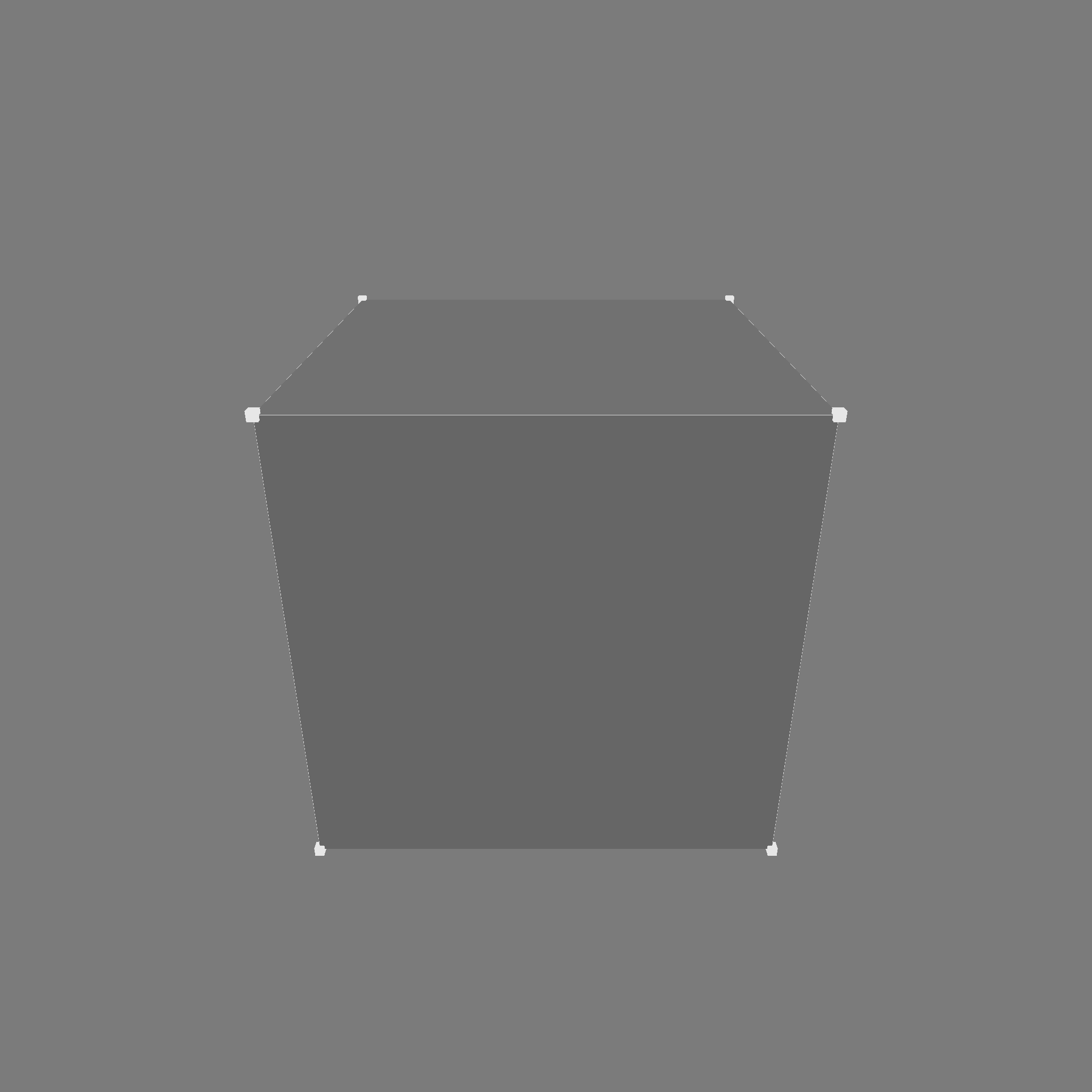
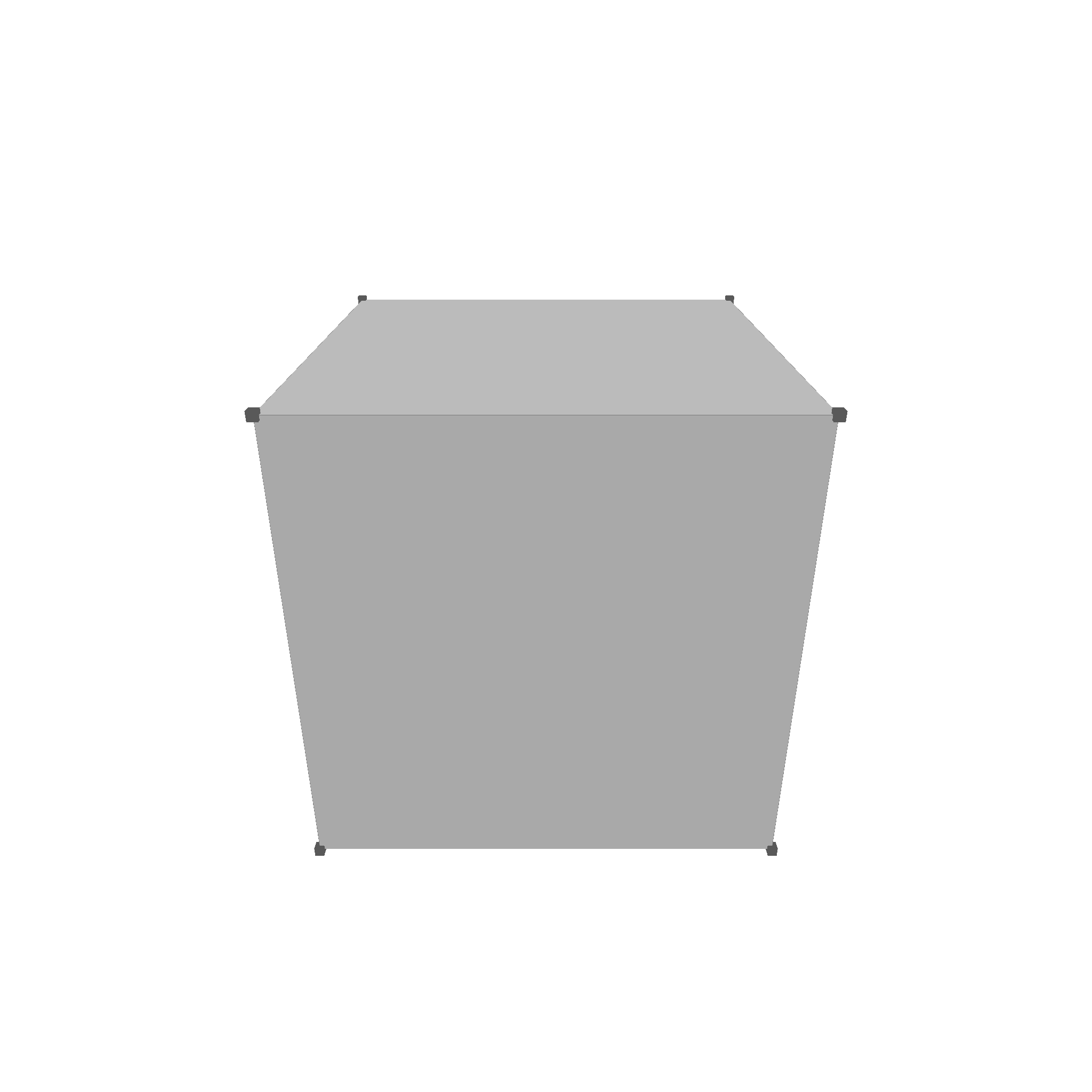
Dark vs light mode

The kernel can be used in both dark and light mode. The following figure shows the difference between the two modes:

Dark mode Light mode

Algebra

The algebra module follows in structure and naming convents the MIT course Shape Interrogation for Computer Aided Design and Manufacturing.

Convex Hull calculation

Convex Hull

EFloat Interval Arithmetic

Lets start with a little fun fact. Did you know, that with f64 floating point numbers, $$0.1 + 0.2 \neq 0.3$$? This is because floating point numbers are not exact. They are approximations. In most programs, it is sufficient to use a small epsilon value to compare floating point numbers. However, in geometric algorithms, we need to be more precise. This is where interval arithmetic comes in.

Geop utilizes the EFloat64 type to represent floating point numbers. It tracks the lower and upper bounds of the floating point number. This allows us to perform arithmetic operations on floating point numbers with a guaranteed error bound. The following testcase magically works. Note how with f64, 0.1 + 0.2 != 0.3, but with EFloat64, 0.1 + 0.2 == 0.3.

#![allow(unused)]
fn main() {
#[test]
fn test_efloat_add() {
    assert!(0.1 + 0.2 != 0.3);
    let a = EFloat64::from(0.1);
    let b = EFloat64::from(0.2);
    let c = a + b;
    println!("c: {:?}", c);
    assert!(c == 0.3);
}
}

Typically, geop will use EFloat64 for all calculations like addition, squareroot, dot products, cross products, etc. which results in an EFloat64 again. As a last step, the EFloat64 is compared to a f64 to determine e.g. if two points intersect. E.g. the following code snipped from the geop-geometry checks if two points are equal:

#![allow(unused)]
fn main() {
impl PartialEq for Point {
    fn eq(&self, other: &Point) -> bool {
        (self.x - other.x) == 0.0 && (self.y - other.y) == 0.0 && (self.z - other.z) == 0.0
    }
}
}

So typically, EFloat64 is used for all calculations, and f64 is only used for comparison. This way, we can guarantee that the error bound is always within a certain range.

Things that return results instead of panicking

There is a couple things which are usually a bad idea:

Dividing by EFloat64. This returns a AlgebraResult. Why? Because of division by zero. If you divide by zero, the result is not a number. So we return a result instead of panicking.
Taking a square root of EFloat64. Well, usually a bad idea, since it is slow, and does not work for negative values.
Normalizing a Point. This returns a AlgebraResult. Why? Because if the point is at the origin, it cannot be normalized. So we return a result instead of panicking.

Why does this matter? Take a look for example at this snipped to check if two homogenous points are equal:

#![allow(unused)]
fn main() {
// equality
impl<T> PartialEq for Homogeneous<T>
where
    T: PartialEq,
{
    fn eq(&self, other: &Self) -> bool {
        (self.point / self.weight).unwrap() == (other.point / other.weight).unwrap()
    }
}
}

Now this panics, if the points weight is 0. Take a look at this implementation instead

#![allow(unused)]
fn main() {
// equality
impl<T> PartialEq for Homogeneous<T>
where
    T: PartialEq,
{
    fn eq(&self, other: &Self) -> bool {
        self.point * other.weight == other.point * self.weight
    }
}
}

This implementation gets the same result, but without needing a division. Thus, it cannot panic, and the implementation is more robust.

People tend to forget to check these edge cases, thus, geop uses the enhanced typing capabilities of Rust, to remind you that a division, or a normalization operation might fail.

Monomial Polynomials

A polynom in monomial representation is of the form $$p(x) = a_0 + a_1 x + a_2 x^2 + \ldots + a_n x^n$$. The monomial representation is a simple list of coefficients. The following code snippet shows the MonomialPolynom struct:

#![allow(unused)]
fn main() {
pub struct MonomialPolynom {
    pub monomials: Vec<EFloat64>,
}
}

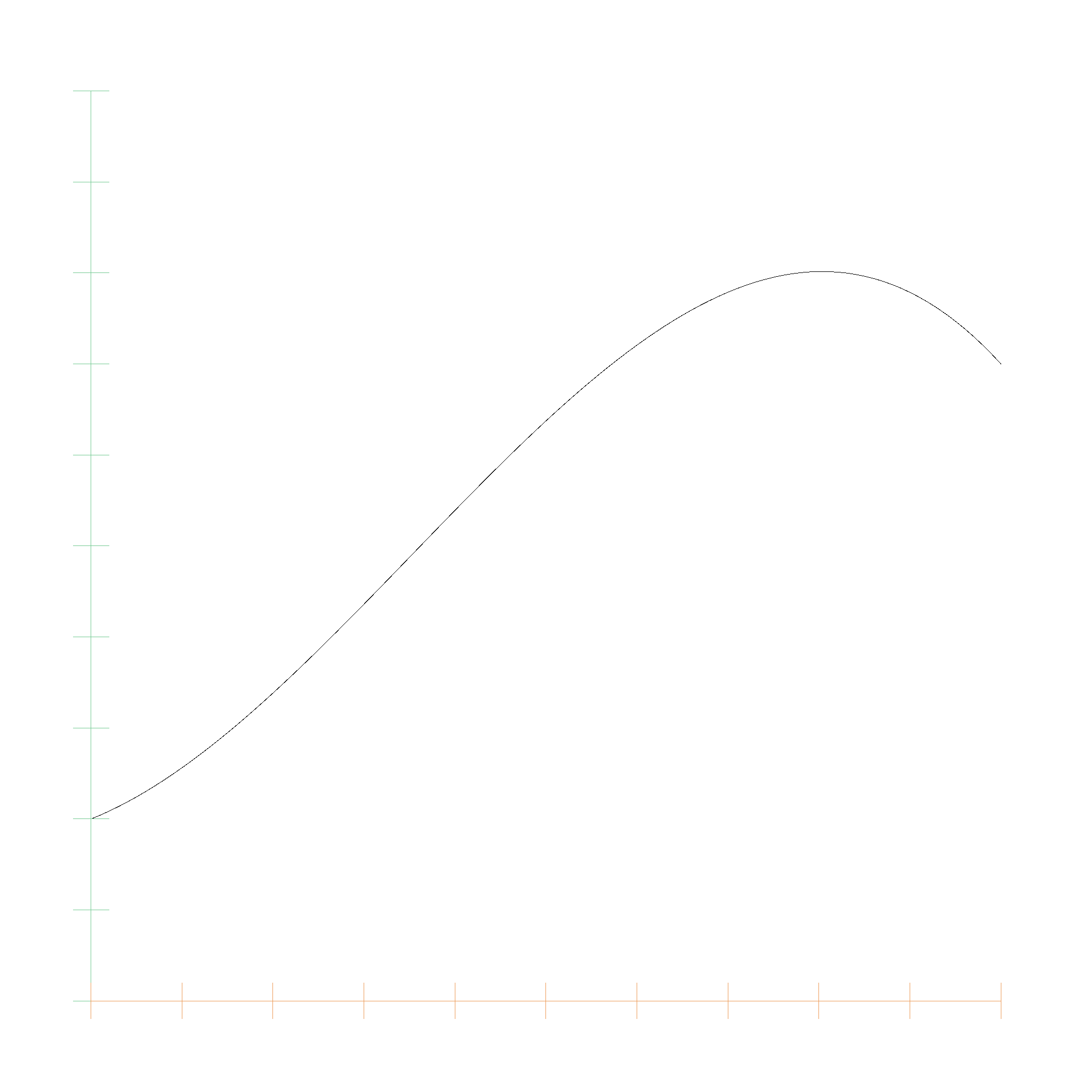
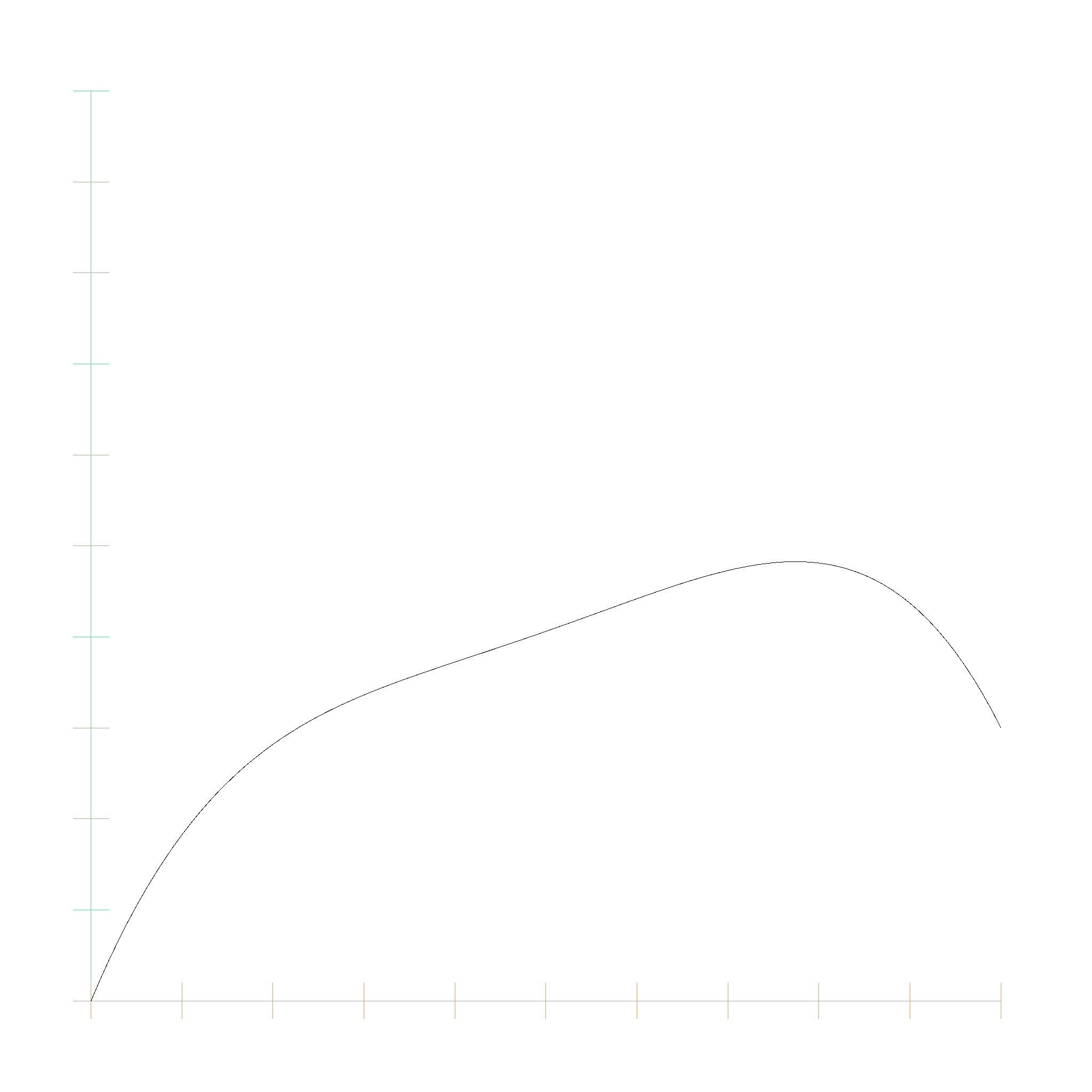
We can add and multiply these polynomials, and use them as algebraic expressions for lines, circles, and so on. This is the plot for

$$p(x) = 0.2 + 0.4 x + 1.8 x^2 -1.7 x^3$$

Monomial Function

Bernstein Polynomials

A polynom in Bernstein representation is of the form $$p(x) = \sum_{i=0}^n a_i B_{i,n}(x)$$, with the basis functions being defined as $$B_{i,n}(x) = \binom{n}{i} x^i (1-x)^{n-i}$$. The Bernstein representation is a list of coefficients, where the coefficients are multiplied with the Bernstein basis functions. The following code snippet shows the BernsteinPolynom struct:

#![allow(unused)]
fn main() {
pub struct BernsteinPolynomial<T> {
    coefficients: Vec<T>,
}
}

Every polynomial can be converted from monomial to Bernstein representation and back. Bernstein Polynomials have better numerical properties than monomial polynomials, and are therefore used in many geometric algorithms.

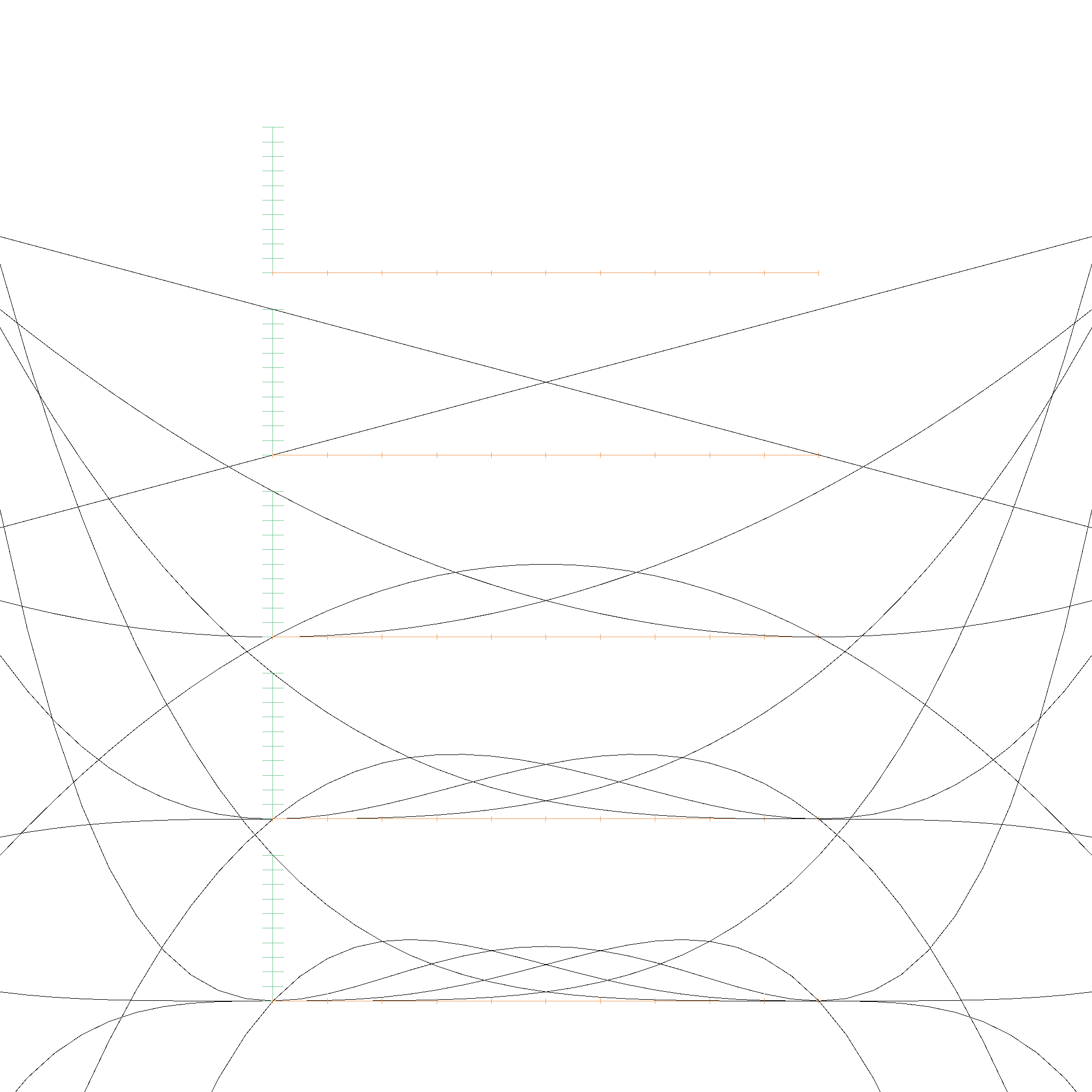
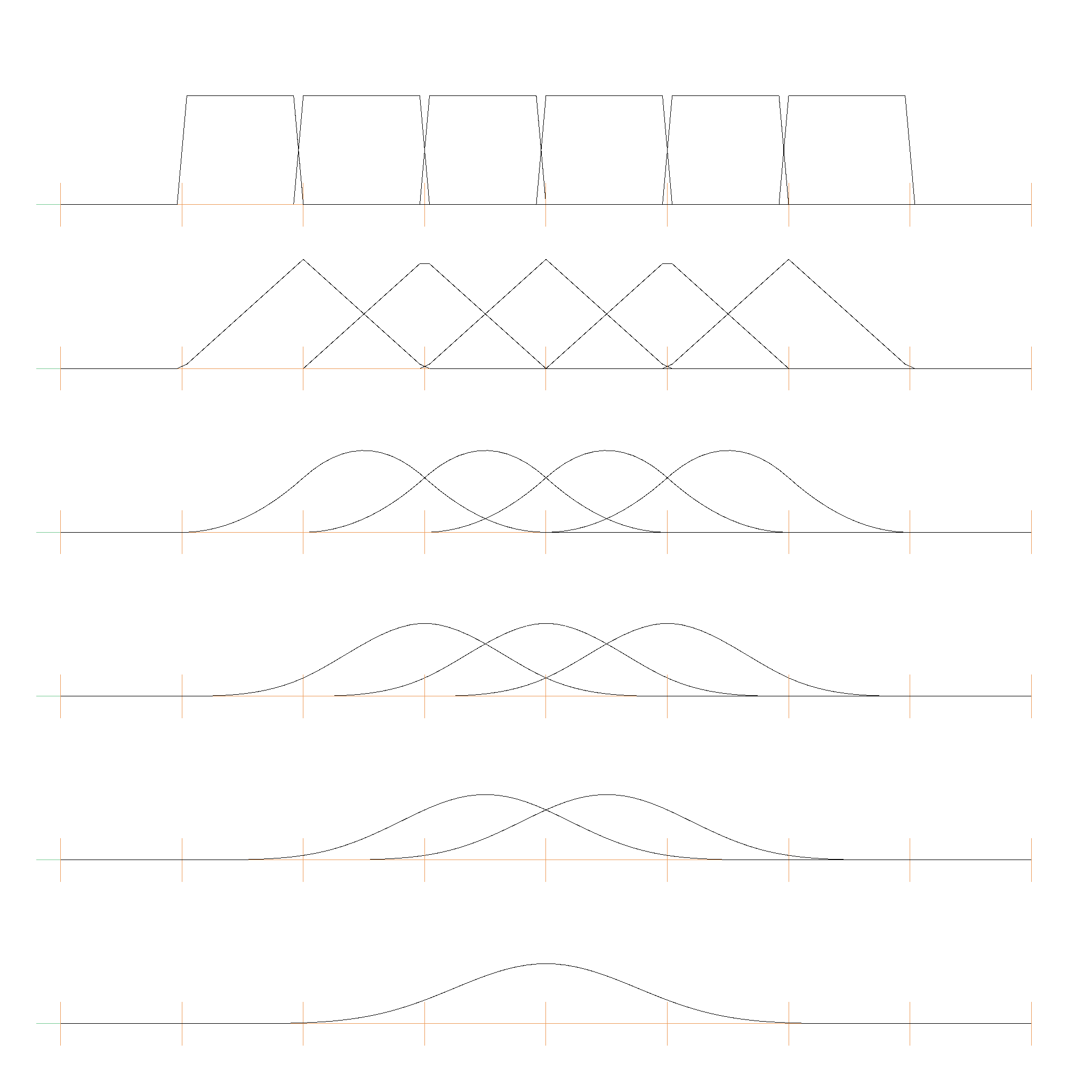
Here is a picture of the Basis functions from $B_{0, 0}$ (top) to $B_{0, 5}$...$B_{5, 5}$ (bottom):

Bernstein Basis Functions

This table lists the polynomial functions $ B_{i,j}(x) $:

$ B_{i,j}(x) $	Expression
$ B_{0,0}(x) $	$ 1.00 \cdot x^0 $
$ B_{0,1}(x) $	$ -1.00 \cdot x^1 + 1.00 \cdot x^0 $
$ B_{1,1}(x) $	$ 1.00 \cdot x^1 $
$ B_{0,2}(x) $	$ 1.00 \cdot x^2 - 2.00 \cdot x^1 + 1.00 \cdot x^0 $
$ B_{1,2}(x) $	$ -2.00 \cdot x^2 + 2.00 \cdot x^1 $
$ B_{2,2}(x) $	$ 1.00 \cdot x^2 $
$ B_{0,3}(x) $	$ -1.00 \cdot x^3 + 3.00 \cdot x^2 - 3.00 \cdot x^1 + 1.00 \cdot x^0 $
$ B_{1,3}(x) $	$ 3.00 \cdot x^3 - 6.00 \cdot x^2 + 3.00 \cdot x^1 $
$ B_{2,3}(x) $	$ -3.00 \cdot x^3 + 3.00 \cdot x^2 $
$ B_{3,3}(x) $	$ 1.00 \cdot x^3 $
$ B_{0,4}(x) $	$ 1.00 \cdot x^4 - 4.00 \cdot x^3 + 6.00 \cdot x^2 - 4.00 \cdot x^1 + 1.00 \cdot x^0 $
$ B_{1,4}(x) $	$ -4.00 \cdot x^4 + 12.00 \cdot x^3 - 12.00 \cdot x^2 + 4.00 \cdot x^1 $
$ B_{2,4}(x) $	$ 6.00 \cdot x^4 - 12.00 \cdot x^3 + 6.00 \cdot x^2 $
$ B_{3,4}(x) $	$ -4.00 \cdot x^4 + 4.00 \cdot x^3 $
$ B_{4,4}(x) $	$ 1.00 \cdot x^4 $
...	...

Many people forget that Bernstein Polynomials are defined on the entire real number range, not just on the interval $[0, 1]$. This means we could extrapolate far beyond the control points, but they spiral out of control quite quickly. However, monomial polynomials are also defined on the entire real number range, so it is nice that we can approximate them entirely with a couple control points.

And this is the Bernstein polynomial with coefficients 0.0, 0.6, 0.1, 0.8, 0.3:

Bernstein Function

Algorithms for polynomials in Bernstein form

There is a great research paper called Algorithms for polynomials in Bernstein form by R.T. Farouki and V.T. Rajan. Most of the following algorithms are based on this paper, which we will quote as Farouki 1988.

Conversion between Monomial and Bernstein

If a polynomial of degree $n$ is given in monomial form and Bernstein form as

$$ P(x) = \sum_{i=0}^n c_i x^i = \sum_{i=0}^n a_{i} B_{i,n}(x) $$

then the coefficients are related by

$$ c_i = \sum_{k=0}^i (-1)^{i - k} \binom{n}{i} \binom{i}{k} a_{k} $$

and

$$ a_i = \sum_{k=0}^i \frac{\binom{i}{k}}{\binom{n}{k}} c_k $$

(Equation 3 Farouki 1988). For example, for $n=4$, the factors for converting to monomial are

1.00e0
-4.00e0 4.00e0
6.00e0  -1.20e1 6.00e0
-4.00e0 1.20e1  -1.20e1 4.00e0
1.00e0  -4.00e0 6.00e0  -4.00e0 1.00e0

and for converting to Bernstein are

1.00e0
1.00e0  2.50e-1
1.00e0  5.00e-1 1.67e-1
1.00e0  7.50e-1 5.00e-1 2.50e-1
1.00e0  1.00e0  1.00e0  1.00e0  1.00e0

Evaluation of Bernstein Polynomials

The evaluation of a Bernstein polynomial is done by the de Casteljau algorithm. The de Casteljau algorithm is a recursive algorithm that evaluates a polynomial at a given point. The algorithm is based on the fact that the Bernstein basis functions are recursively defined. The algorithm is as follows:

#![allow(unused)]
fn main() {
impl<T> BernsteinPolynomial<T> {
    fn eval(&self, t: EFloat64) -> T {
        let mut beta = self.coefficients.clone();
        let n = beta.len();
        for j in 1..n {
            for k in 0..n - j {
                beta[k] = beta[k].clone() * (EFloat64::one() - t.clone())
                    + beta[k + 1].clone() * t.clone();
            }
        }
        beta[0].clone()
    }
}
}

This is described in Wikipedia.

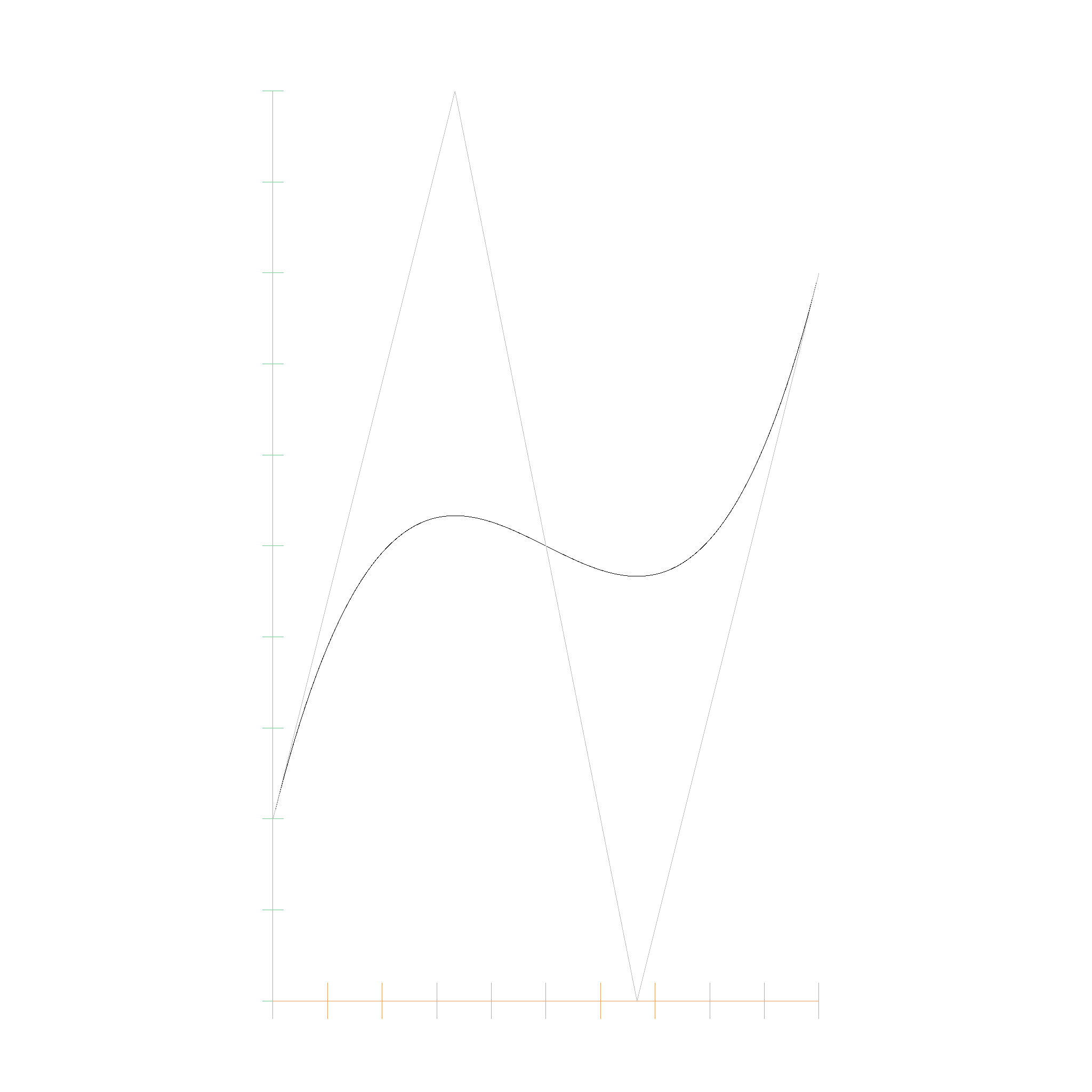
Subdivision

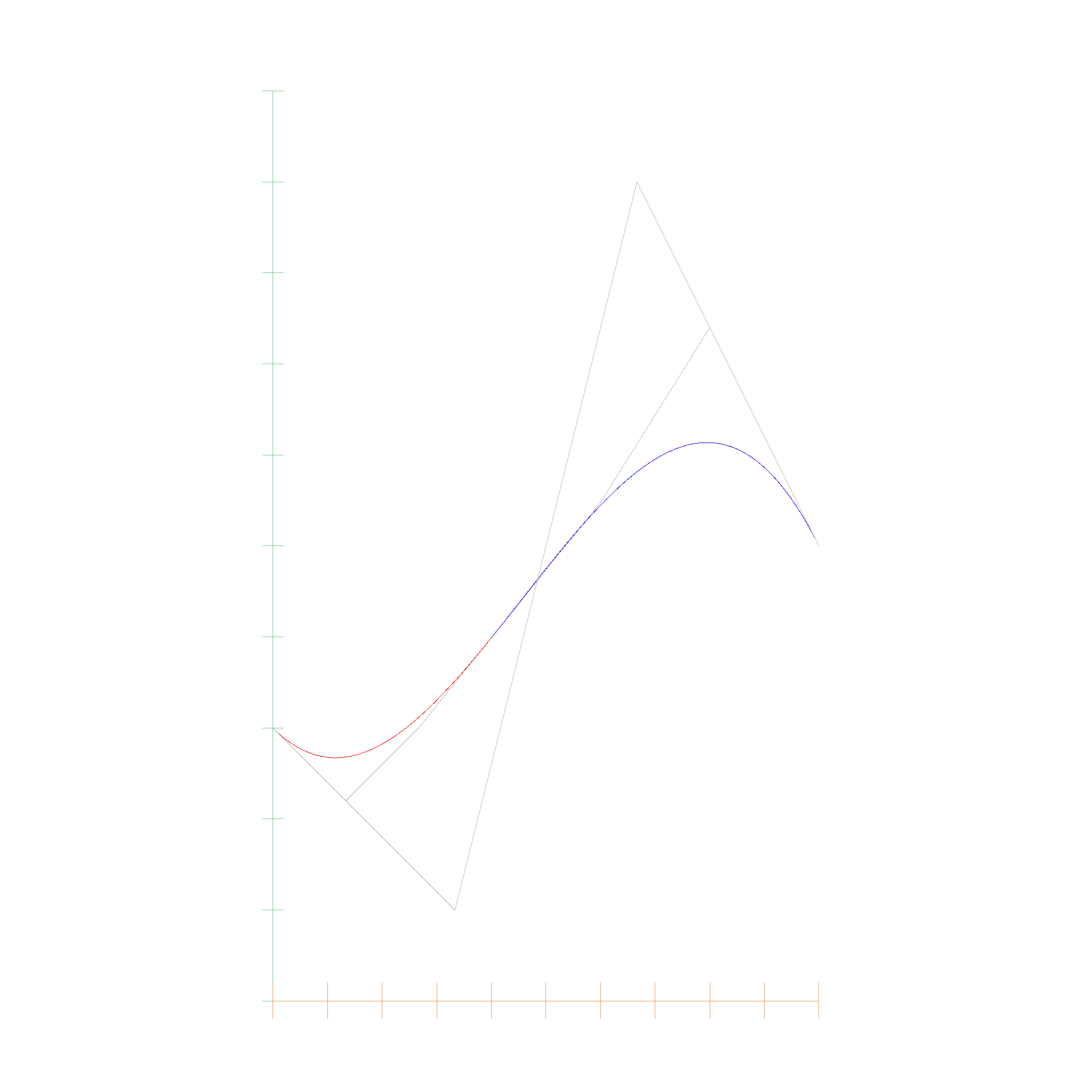
Interestingly, the betas which are computed in the de Casteljau algorithm can also be used to subdivide the polynomial. The MIT Course has a nice visualization of this process.

The betas form a pyramid, where the base (left in the image) is the original polynomial, and the top (right in the image) is the polynomial evaluated at $t$. The subdivision is done by taking the left border of the pyramid and the right border of the pyramid, which are the two polynomials evaluated at $t$, and the middle border, which is the polynomial evaluated at $t/2$. Here you can see how the polynomial is subdivided into two polynomials, the red and the blue one:

Subdivision

Root finding

Here comes the fun part: Now that we can subdivide a bernstein polynomial, we can use it to find roots. Using Bézout's theorem, we know that a polynomial has either infinitely many roots, or a finite number of roots.

If the polynomial has infinitely many roots, then the polynomial is the zero polynomial.
Otherwise, the polynomial has a finite number of roots.

Next, we use the convex hull property of Bernstein Polynomials. The convex hull of a Bernstein Polynomial is the convex hull of the control points. If the convex hull of the control points does not contain the x-axis, then the polynomial has no roots. If the convex hull has both positive and negative y-values, then the polynomial may have roots.

This results in a very simple algorithm to find the roots of a polynomial in interval arithmetic:

Check if the coefficients are all definetly positive or all negative. If they are, then the polynomial has no roots.
Otherwise, subdivide the polynomial in the middle into left and right side:
- If for one side, all coefficients contain 0, we have reached the limits of numerical precision and can return the interval as a root.
- Otherwise, subdivide the polynomial again.
- When merging the roots of two subdivided intervals, we have to check if the last root of the left interval overlaps with the first root of the right interval. If they overlap, then we have to merge them into one root.

The nice part is, that this algorithm does not require an initial guess, or some predetermined accuracy for stopping the algorithm. The algorithm will always find all roots, and will always find the roots with the highest possible accuracy, and will make sure that a single root is not counted multiple times.

Root Finding

Root: EFloat64 { upper_bound: 0.09129127973297148, lower_bound: 0.09129127973297078 }
Root: EFloat64 { upper_bound: 0.20542974361061986, lower_bound: 0.20542974361061803 }
Root: EFloat64 { upper_bound: 0.5130593945291194, lower_bound: 0.5130593945291179 }
Root: EFloat64 { upper_bound: 0.7941467075365286, lower_bound: 0.7941467075365266 }

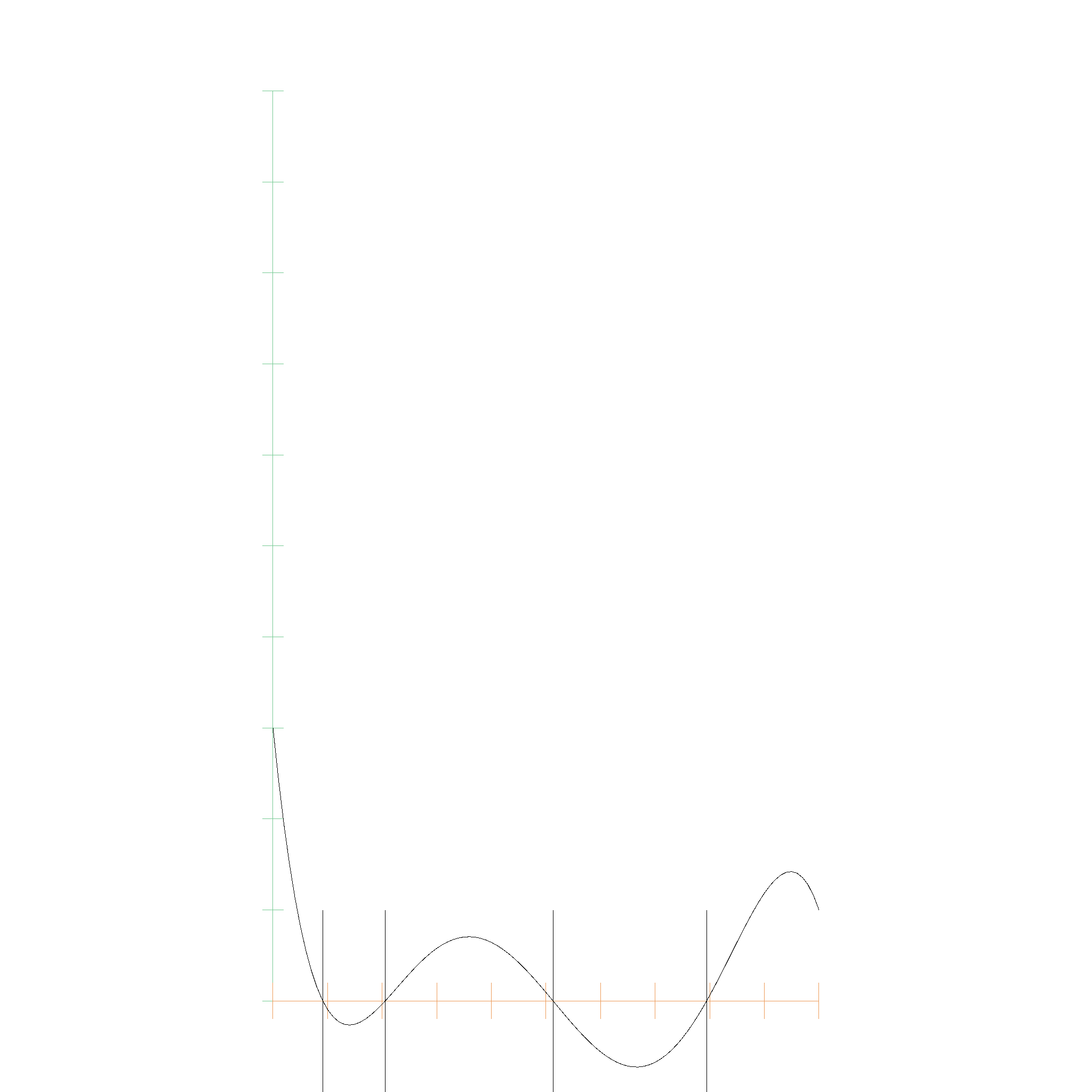
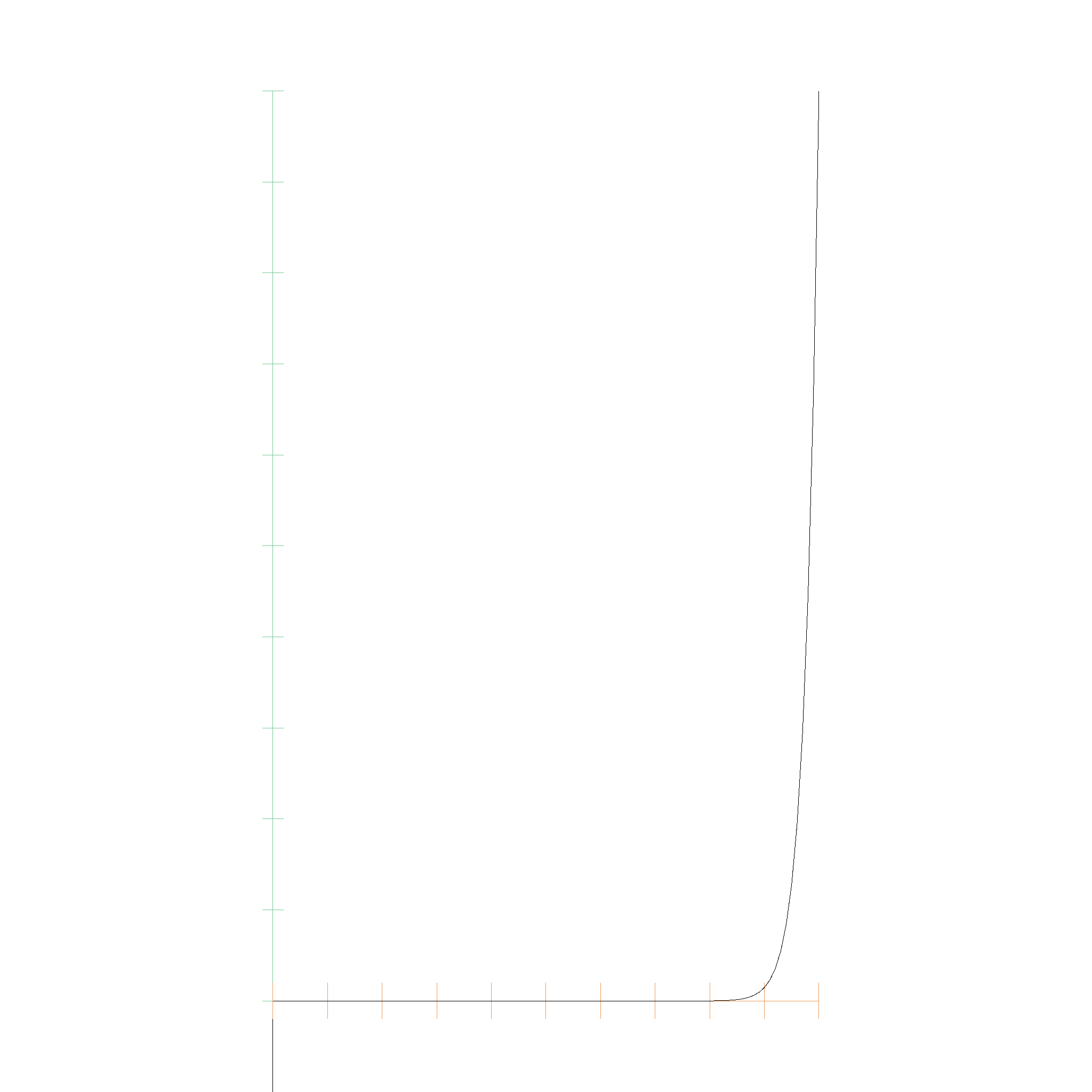
This algorithm converges fast, even for nasty polynomials. This, for example is a polynomial with the first 9 coefficients being 0.0, and the 10th coefficient being 1.0:

running 1 test
t_min: 0, t_max: 1
t_min: 0, t_max: 0.5
t_min: 0, t_max: 0.25
t_min: 0, t_max: 0.125
t_min: 0, t_max: 0.0625
t_min: 0, t_max: 0.03125
t_min: 0, t_max: 0.015625
t_min: 0, t_max: 0.0078125
t_min: 0, t_max: 0.00390625
t_min: 0, t_max: 0.001953125
t_min: 0, t_max: 0.0009765625
t_min: 0, t_max: 0.00048828125
t_min: 0, t_max: 0.000244140625
t_min: 0, t_max: 0.0001220703125
t_min: 0, t_max: 0.00006103515625
t_min: 0, t_max: 0.000030517578125
t_min: 0, t_max: 0.0000152587890625
t_min: 0, t_max: 0.00000762939453125
t_min: 0, t_max: 0.000003814697265625
t_min: 0, t_max: 0.0000019073486328125
t_min: 0, t_max: 0.00000095367431640625
t_min: 0, t_max: 0.000000476837158203125
t_min: 0, t_max: 0.0000002384185791015625
t_min: 0, t_max: 0.00000011920928955078125
t_min: 0, t_max: 0.00000005960464477539063
t_min: 0, t_max: 0.000000029802322387695313
t_min: 0, t_max: 0.000000014901161193847656
t_min: 0, t_max: 0.000000007450580596923828
t_min: 0, t_max: 0.000000003725290298461914
t_min: 0, t_max: 0.000000001862645149230957
t_min: 0, t_max: 0.0000000009313225746154785
t_min: 0, t_max: 0.0000000004656612873077393
t_min: 0, t_max: 0.00000000023283064365386963
t_min: 0, t_max: 0.00000000011641532182693481
t_min: 0, t_max: 0.00000000005820766091346741
t_min: 0, t_max: 0.000000000029103830456733704
t_min: 0, t_max: 0.000000000014551915228366852
t_min: 0, t_max: 0.000000000007275957614183426
t_min: 0, t_max: 0.000000000003637978807091713
t_min: 0, t_max: 0.0000000000018189894035458565
t_min: 0, t_max: 0.0000000000009094947017729282
t_min: 0, t_max: 0.0000000000004547473508864641
t_min: 0, t_max: 0.00000000000022737367544323206
t_min: 0, t_max: 0.00000000000011368683772161603
t_min: 0, t_max: 0.00000000000005684341886080802
t_min: 0, t_max: 0.00000000000002842170943040401
t_min: 0, t_max: 0.000000000000014210854715202004
t_min: 0, t_max: 0.000000000000007105427357601002
t_min: 0, t_max: 0.000000000000003552713678800501
t_min: 0, t_max: 0.0000000000000017763568394002505
t_min: 0, t_max: 0.0000000000000008881784197001252
t_min: 0, t_max: 0.0000000000000004440892098500626
t_min: 0, t_max: 0.0000000000000002220446049250313
t_min: 0, t_max: 0.00000000000000011102230246251565
t_min: 0, t_max: 0.00000000000000005551115123125783
t_min: 0, t_max: 0.000000000000000027755575615628914
t_min: 0, t_max: 0.000000000000000013877787807814457
t_min: 0, t_max: 0.000000000000000006938893903907228
t_min: 0, t_max: 0.000000000000000003469446951953614
t_min: 0, t_max: 0.000000000000000001734723475976807
t_min: 0, t_max: 0.0000000000000000008673617379884035
t_min: 0, t_max: 0.0000000000000000004336808689942018
t_min: 0, t_max: 0.0000000000000000002168404344971009
t_min: 0, t_max: 0.00000000000000000010842021724855044
t_min: 0, t_max: 0.00000000000000000005421010862427522
t_min: 0, t_max: 0.00000000000000000002710505431213761
t_min: 0, t_max: 0.000000000000000000013552527156068805
t_min: 0, t_max: 0.000000000000000000006776263578034403
t_min: 0, t_max: 0.0000000000000000000033881317890172014
t_min: 0, t_max: 0.0000000000000000000016940658945086007
t_min: 0, t_max: 0.0000000000000000000008470329472543003
t_min: 0, t_max: 0.0000000000000000000004235164736271502
t_min: 0, t_max: 0.0000000000000000000002117582368135751
t_min: 0, t_max: 0.00000000000000000000010587911840678754
t_min: 0, t_max: 0.00000000000000000000005293955920339377
t_min: 0, t_max: 0.000000000000000000000026469779601696886
t_min: 0, t_max: 0.000000000000000000000013234889800848443
t_min: 0, t_max: 0.000000000000000000000006617444900424222
t_min: 0, t_max: 0.000000000000000000000003308722450212111
t_min: 0, t_max: 0.0000000000000000000000016543612251060553
t_min: 0, t_max: 0.0000000000000000000000008271806125530277
t_min: 0, t_max: 0.00000000000000000000000041359030627651384
t_min: 0, t_max: 0.00000000000000000000000020679515313825692
t_min: 0, t_max: 0.00000000000000000000000010339757656912846
t_min: 0, t_max: 0.00000000000000000000000005169878828456423
t_min: 0, t_max: 0.000000000000000000000000025849394142282115
t_min: 0, t_max: 0.000000000000000000000000012924697071141057
t_min: 0, t_max: 0.000000000000000000000000006462348535570529
t_min: 0, t_max: 0.0000000000000000000000000032311742677852644
t_min: 0, t_max: 0.0000000000000000000000000016155871338926322
t_min: 0, t_max: 0.0000000000000000000000000008077935669463161
t_min: 0, t_max: 0.00000000000000000000000000040389678347315804
t_min: 0, t_max: 0.00000000000000000000000000020194839173657902
t_min: 0, t_max: 0.00000000000000000000000000010097419586828951
t_min: 0, t_max: 0.00000000000000000000000000005048709793414476
t_min: 0, t_max: 0.00000000000000000000000000002524354896707238
t_min: 0, t_max: 0.00000000000000000000000000001262177448353619
t_min: 0, t_max: 0.000000000000000000000000000006310887241768095
t_min: 0, t_max: 0.0000000000000000000000000000031554436208840472
t_min: 0, t_max: 0.0000000000000000000000000000015777218104420236
t_min: 0, t_max: 0.0000000000000000000000000000007888609052210118
t_min: 0, t_max: 0.0000000000000000000000000000003944304526105059
t_min: 0, t_max: 0.00000000000000000000000000000019721522630525295
t_min: 0, t_max: 0.00000000000000000000000000000009860761315262648
t_min: 0, t_max: 0.00000000000000000000000000000004930380657631324
t_min: 0, t_max: 0.00000000000000000000000000000002465190328815662
t_min: 0, t_max: 0.00000000000000000000000000000001232595164407831
t_min: 0, t_max: 0.000000000000000000000000000000006162975822039155
t_min: 0, t_max: 0.0000000000000000000000000000000030814879110195774
t_min: 0, t_max: 0.0000000000000000000000000000000015407439555097887
t_min: 0, t_max: 0.0000000000000000000000000000000007703719777548943
t_min: 0, t_max: 0.0000000000000000000000000000000003851859888774472
t_min: 0, t_max: 0.0000000000000000000000000000000001925929944387236
t_min: 0, t_max: 0.0000000000000000000000000000000000962964972193618
t_min: 0, t_max: 0.0000000000000000000000000000000000481482486096809
t_min: 0, t_max: 0.00000000000000000000000000000000002407412430484045
t_min: 0, t_max: 0.000000000000000000000000000000000012037062152420224
t_min: 0, t_max: 0.000000000000000000000000000000000006018531076210112
t_min: 0, t_max: 0.000000000000000000000000000000000003009265538105056

Root Finding

The following one is even nastier, with 39 coefficients being 0.0, and the 40th coefficient being 1.0. The algorithm stops faster, as its running into numerical limitations faster. This results in the root being less accurate, but still as accurate as possible with the given floating point precision:

t_min: 0, t_max: 1
t_min: 0, t_max: 0.5
t_min: 0, t_max: 0.25
t_min: 0, t_max: 0.125
t_min: 0, t_max: 0.0625
t_min: 0, t_max: 0.03125
t_min: 0, t_max: 0.015625
t_min: 0, t_max: 0.0078125
t_min: 0, t_max: 0.00390625
t_min: 0, t_max: 0.001953125
t_min: 0, t_max: 0.0009765625
t_min: 0, t_max: 0.00048828125
t_min: 0, t_max: 0.000244140625
t_min: 0, t_max: 0.0001220703125
t_min: 0, t_max: 0.00006103515625
t_min: 0, t_max: 0.000030517578125
t_min: 0, t_max: 0.0000152587890625
t_min: 0, t_max: 0.00000762939453125
t_min: 0, t_max: 0.000003814697265625
t_min: 0, t_max: 0.0000019073486328125
t_min: 0, t_max: 0.00000095367431640625
t_min: 0, t_max: 0.000000476837158203125
t_min: 0, t_max: 0.0000002384185791015625
t_min: 0, t_max: 0.00000011920928955078125
t_min: 0, t_max: 0.00000005960464477539063
t_min: 0, t_max: 0.000000029802322387695313
t_min: 0, t_max: 0.000000014901161193847656

Root Finding

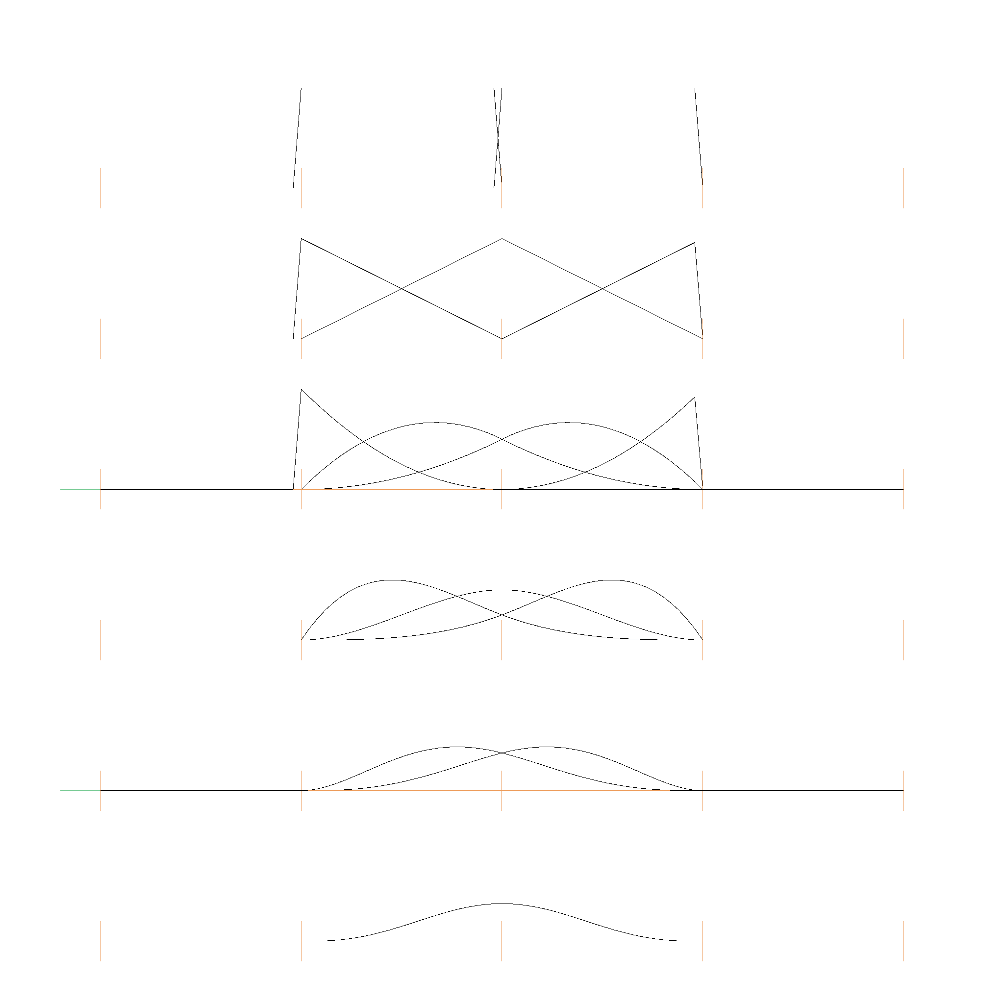
Degree Elevation

Equation 27 of Farouki 1988 describes how to elevate the degree of a Bernstein polynomial. The new coefficients are given by

$$ c_i^{n+r} = \sum_{j = max(0, i - r)}^{min(n, i)} \frac{\binom{r}{i - j} \binom{n}{j}}{\binom{n + r}{i}} c_i^n $$

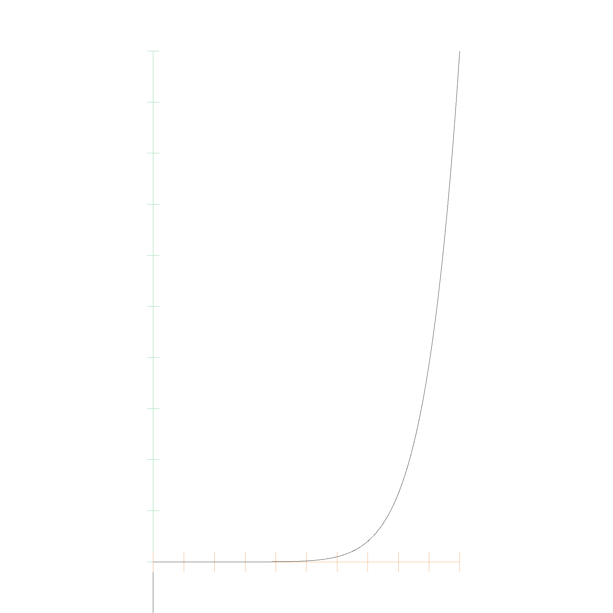
Here is an example of degree elevation from degree 1 to 3:

Bernstein Polynomial: 1.00e0 B_{0,1}(t) + 2.00e0 B_{1,1}(t)
Elevated Bernstein Polynomial: 1.00e0 B_{0,2}(t) + 1.50e0 B_{1,2}(t) + 2.00e0 B_{2,2}(t)
Elevated Bernstein Polynomial 2: 1.00e0 B_{0,3}(t) + 1.33e0 B_{1,3}(t) + 1.67e0 B_{2,3}(t) + 2.00e0 B_{3,3}(t)

Bezier curves

If we use a Bernstein Polynomial with Points instead of EFloats for the coefficients, we get a Bezier Curve.

Bezier Curve

B Splines

B-Splines are slightly different from Bernstein Polynomials and Bezier Curves.

The B-Spline basis functions are defined recursively as follows:

$$ N_{i,0}(t) = \begin{cases} 1 & \text{if } t_i \leq t < t_{i+1}\\ 0 & \text{otherwise} \end{cases} $$

$$ N_{i,k}(t) = \frac{t - t_i}{t_{i+k} - t_i} N_{i,k-1}(t) + \frac{t_{i+k+1} - t}{t_{i+k+1} - t_{i+1}} N_{i+1,k-1}(t) $$

where $t_i$ are the knot values. The know values can be strictly increasing or non-decreasing. Here is an example for strictly increasing knot values [0, 1, 2, 3, 4, 5, 6, 7]:

B-Spline Basis Functions

And here is one for non-decreasing knot values [0, 0, 0, 1, 2, 2, 2]:

B-Spline Basis Functions

A b-spline curve is defined as:

$$ C(t) = \sum_{i=0}^{n} P_i N_{i,k}(t) $$

where $P_i$ are the control points.

Nurbs

Here are some nurbs

Nurbs Nurbs

Root finding

Root finding with algebraic expressions

Why do we care so much about algebraic expressions like Bernstein Polynomials or Nurbs? Because using the IPP (Interval Projected Polyhedro Algorithm) allows us to find arbitrary roots of them. Let's consider the following example:

Imagine there is a line

$$p(t) = \vec{a} + t \vec{b}$$

And a circle in its implicit form (intersection of a sphere and a plane):

$$u_1(x, y, z) = x ^ 2 + y ^ 2 + z ^ 2 - r = 0$$ $$u_2(x, y, z) = n_1 x + n_2 y + n_3 z = 0$$

Now to find the intersection, we have to solve

$$u_1(p(t)) = 0$$ $$u_2(p(t)) = 0$$

This is a system of equations which is polynomial in nature. We can solve multiple systems of polynomial equations with IPP.

Curve curve intersection

This is a table to show which roots to find depending on if the curve is explicit or implicit:

Curve 1	Curve 2	Roots to find
Implicit $u_1, u_2$	Implicit $v_1, v_2$	$u_1(x, y, z) = 0, u_2(x, y, z) = 0, v_1(x, y, z) = 0, v_2(x, y, z) = 0$
Implicit $u_1, u_2$	Explicit $p(t_2)$	$u_1(p(t_2)) = 0, u_2(p(t_2)) = 0$
Explicit $p(t_1)$	Explicit $p(t_2)$	$p(t_1) - p(t_2) = 0$

Since we can add, multiply and compose algebraic expressions, we can easily find the intersection of two curves. We just setup the "Roots to find" equation and let the IPP algorithm do the rest.

We expect the solution to be either a curve (if the curves are equal), or a set of points.

Curve surface intersection

Curve 1	Surface 2	Roots to find
Implicit $u_1, u_2$	Implicit $v_1$	$u_1(x, y, z) = 0, u_2(x, y, z) = 0, v_1(x, y, z) = 0$
Implicit $u_1, u_2$	Explicit $p(t_2, t_3)$	$u_1(p(t_3, t_4)) = 0, u_2(p(t_3, t_4)) = 0$
Explicit $p(t_1)$	Implicit $v_1$	$v_1(p(t_1)) = 0$
Explicit $p(t_1)$	Explicit $p(t_2, t_3)$	$p(t_1) - p(t_2, t_3) = 0$

We expect the solution to be either a curve (if the curve is embedded in the surface), or a set of points.

Surface surface intersection

Surface 1	Surface 2	Roots to find
Implicit $u_1$	Implicit $v_1$	$u_1(x, y, z) = 0, v_1(x, y, z) = 0$
Implicit $u_1$	Explicit $p(t_3, t_4)$	$u_1(p(t_3, t_4)) = 0$
Explicit $p(t_1, t_2)$	Explicit $p(t_3, t_4)$	$p(t_1, t_2) - p(t_3, t_4) = 0$

We expect the solution to be either a surface (if the two surfaces are equal), or a set of points and curves.

Root finding

Now that we have a "roots to find" equation for each intersection type, we can use our favorite root finding algorithm.

For the curve-curve intersection, we can first check for equality, and if we ruled out equality, we can use IPP to find all intersection points.
For the curve-surface intersection, we can first check for containment, and if we ruled out containment, IPP will tell us the points.
For the surface-surface intersection, things get more complicated. If the surfaces are equal, we can simply return the surface. But if they differ, we have to find all numerical approximations of the intersection curves, or tell the solver, which curve should be fittet to the solution (e.g. with two spheres, we know that we have the solution should look like a circle).

Root finding algorithms for points

Newton-Raphson

For benchmarking, we implement the Newton-Raphson method. It is very easy to implement. However, it is not guaranteed to find all roots, since we have to use an initial guess.

IPP Algorithm

The standard algorithm used for root finding is the IPP algorithm. How the IPP algorithm works is explained in the Interval Projected Polyhedron Algorithm section of the MIT course. It will always find all roots.

Root finding algorithms for curves

There is an idea on how to modify IPP to to deal with curves, and return Bernstein Polynomials / Nurbs with bounded errors to the true solution, but it will be tough to implement.

The polygon used to represent the boundary of the root will start to shrink towards a line, if the solution is a curve. We have to recognize this, and limit the shrinking along the main axis, but shrink along the perpendicular intersection axis as far as possible.

A second step could be the fitting of a closed form solution (e.g. a circle) to the approximation.

Geometry

Geometry refers to structures that represent unbounded / inifinite objects, like planes, spheres, circles, lines, etc. These objects are used to define the shape of the objects in the scene. The simples case are curves.

Curves

A curve is something that could be thought of as a function that maps a number to a point in space. Right now, geop implements only two primitive curves. This is a line, defined by a basis and a direction.

#![allow(unused)]
fn main() {
let line = Line::new(
    Point3::new(0.0, 0.0, 0.0),
    Point3::new(1.0, 0.0, 0.0),
);
}

Line

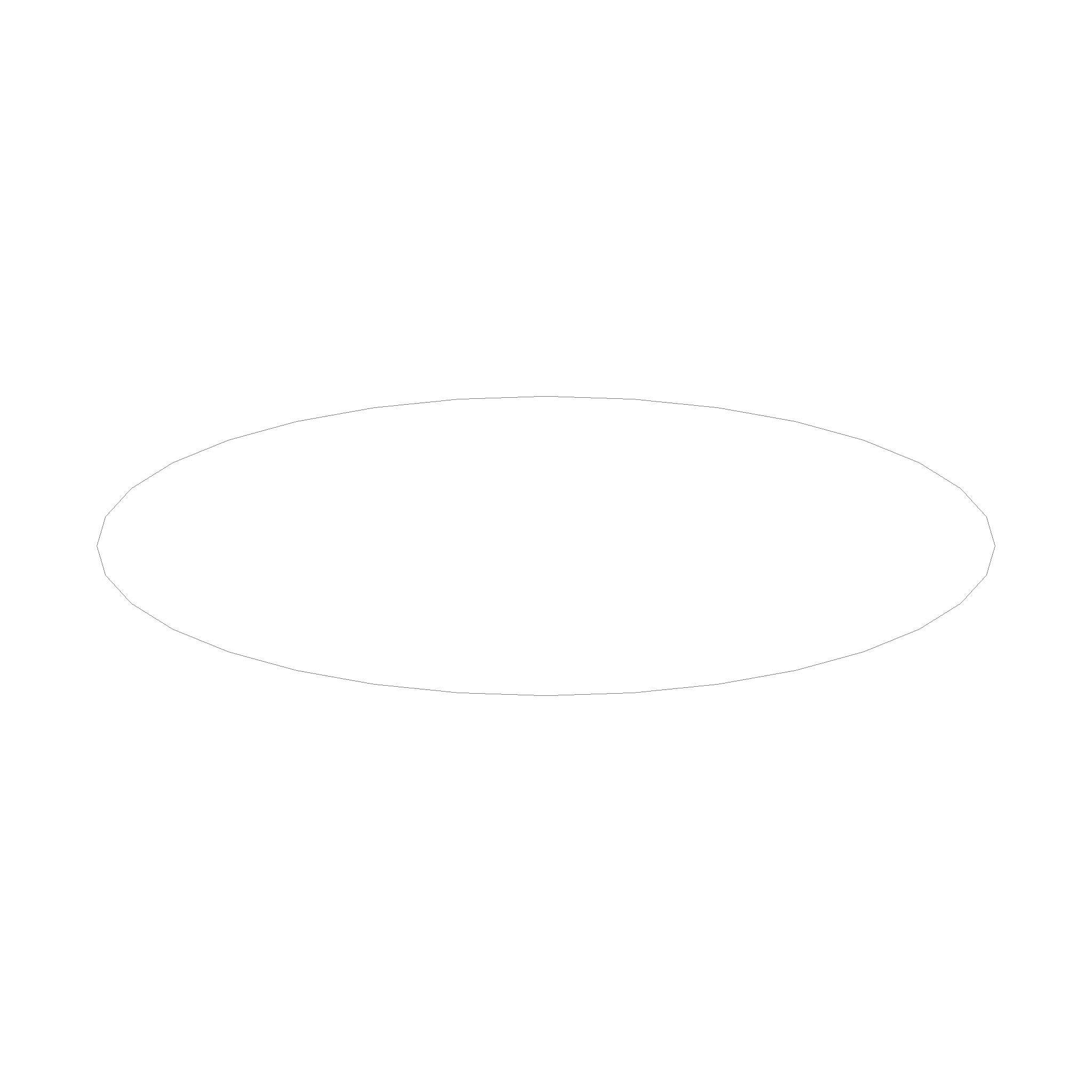
Next is a circle, defined by a center, a normal and a radius. The radius is a point, indicating where the circle starts or is at 0.

#![allow(unused)]
fn main() {
let circle = Circle::new(
    Point3::new(0.0, 0.0, 0.0),
    Point3::new(0.0, 0.0, 1.0),
    1.0,
);
}

Circle

There is an ellipsis.

#![allow(unused)]
fn main() {
let ellipsis = Ellipsis::new(
    Point3::new(0.0, 0.0, 0.0),
    Point3::new(0.0, 1.0, 0.0),
    Point3::new(1.0, 0.0, 0.0),
    Point3::new(0.0, 0.0, 1.0),
);
}

Ellipsis

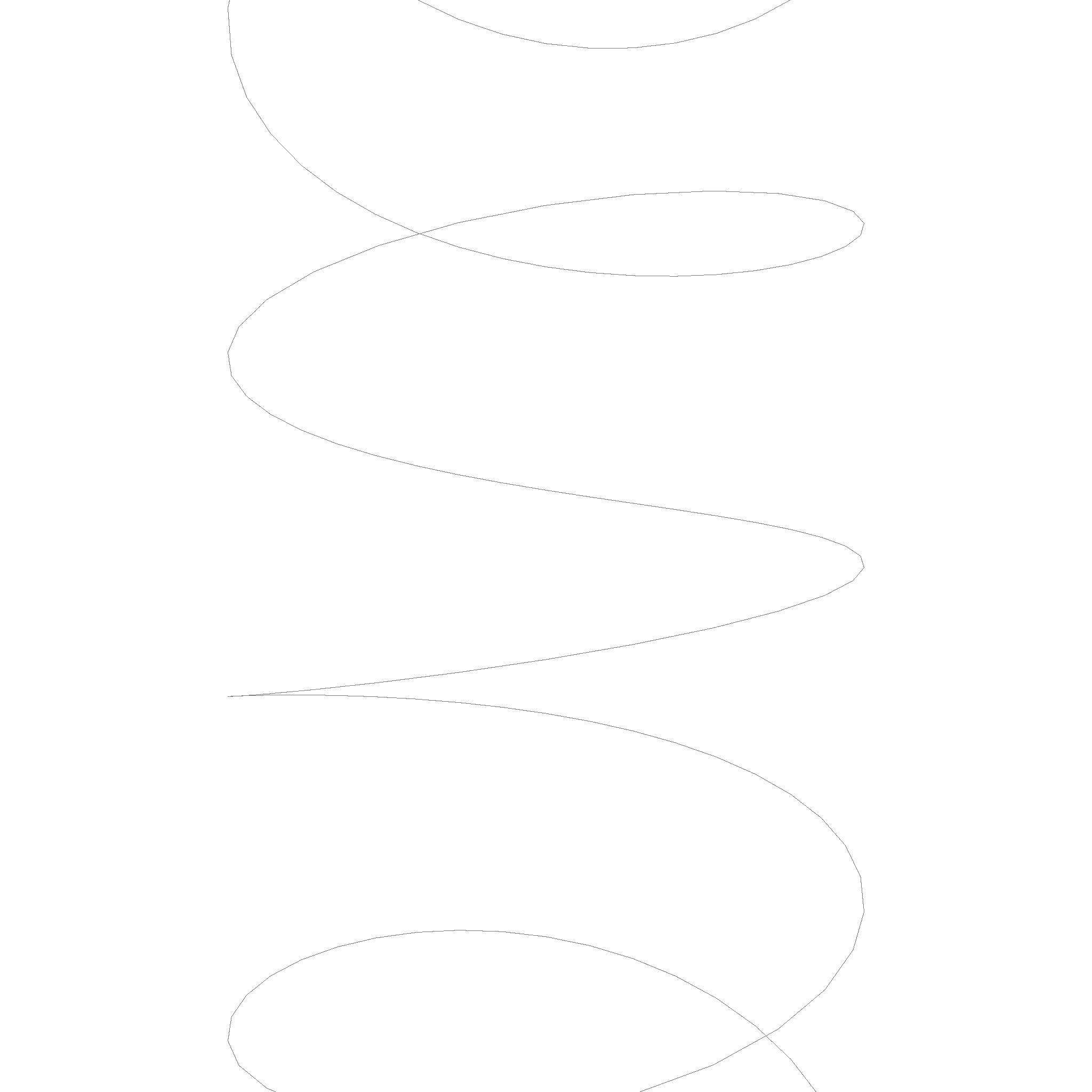
There are also more interesting curves, like a Helix.

#![allow(unused)]
fn main() {
let helix = Helix::new(
    Point3::new(0.0, 0.0, 0.0),
    Point3::new(0.0, 0.0, 1.0),
    Point3::new(1.0, 0.0, 0.0),
);
}

Helix

Do not expose the parameters

Technically, all the curves are something like $$c(u): \mathbb{R} \rightarrow \mathbb{R}^3, u \rightarrow p$$ But we don't want to use the parameters, as they are very dangerous and misleading in general. For example, imagine writing a function that checks if a point is in an interval. You would write something like this:

#![allow(unused)]
fn main() {
// Checks if p is between a and b
fn is_in_interval(p: Point3, a: Point3, b: Point3) -> bool {
    let u_p = unproject(p);
    let u_a = unproject(a);
    let u_b = unproject(b);
    u_p >= u_a && u_p <= u_b
}
}

However, this code does not work for a circle. A circle has no unique mapping from $p$ to $u$. So, we have to avoid using the parameters. This is why the curves do not expose the parameters.

How to interact with curves

How do we interact with curves? We can do this by using the Curve trait. It implements the following methods:

#![allow(unused)]
fn main() {
// Transform
pub fn transform(&self, transform: Transform) -> Curve;

// Change the direction of the curve
pub fn neg(&self) -> Curve;

// Normalized Tangent / Direction of the curve at the given point.
pub fn tangent(&self, p: Point) -> Point;

// Checks if point is on the curve.
pub fn on_curve(&self, p: Point) -> bool;

// Interpolate between start and end at t. t is between 0 and 1.
pub fn interpolate(&self, start: Option<Point>, end: Option<Point>, t: f64) -> Point;

// Checks if m is between x and y. m==x and m==y are true.
pub fn between(&self, m: Point, start: Option<Point>, end: Option<Point>) -> bool;

// Get the midpoint between start and end.
// This will guarantee that between(start, midpoint, end) is true and midpoint != start and midpoint != end.
// If start or end is None, the midpoint is a point that is a unit distance away from the other point.
pub fn get_midpoint(&self, start: Option<Point>, end: Option<Point>) -> Point;

// Finds the closest point on the curve to the given point.
pub fn project(&self, p: Point) -> Point;
}

These are all the methods that have to be used to interact with curves. You might notice, that interpolate, between and get_midpoint functions accept Optional. This is for cases where we work with infinite edges. For example, a line that starts somewhere and goes to infinity would work with start = Some(Point3::new(0.0, 0.0, 0.0)) and end = None. Circles also frequently don't have a start and end point.

Intersections

Intersections are fully supported between all curves. Keep in mind, that intersections are not always a single point. For example, two lines can intersect in one point, but they can also intersect in infinitely many points if they are the same line, or in no points if they are parallel. This is represented by the enum data type that is returned by the intersection function.

#![allow(unused)]
fn main() {
#[derive(Debug)]
pub enum CircleCircleIntersection {
    Circle(Circle),
    TwoPoint(Point, Point),
    OnePoint(Point),
    None,
}

pub fn circle_circle_intersection(a: &Circle, b: &Circle) -> CircleCircleIntersection;
}

Interestingly, there are no cases where the intersection of two curves results in a curve and a point.

Note: The intersection of two curves is EITHER a curve OR a list of points OR nothing. There is no case where the intersection is a curve and a point, or a bounded curve.

#![allow(unused)]
fn main() {
pub enum CurveCurveIntersection {
    None,
    Points(Vec<Point>),
    Curve(Curve),
}

pub fn curve_curve_intersection(edge_self: &Curve, edge_other: &Curve) -> CurveCurveIntersection;
}

This property also extends to more complicated geometries like nurbs and means these datastructures are well closed under intersection. This also explains why they reside in their own crate. We use this property many times later in the topology modules.

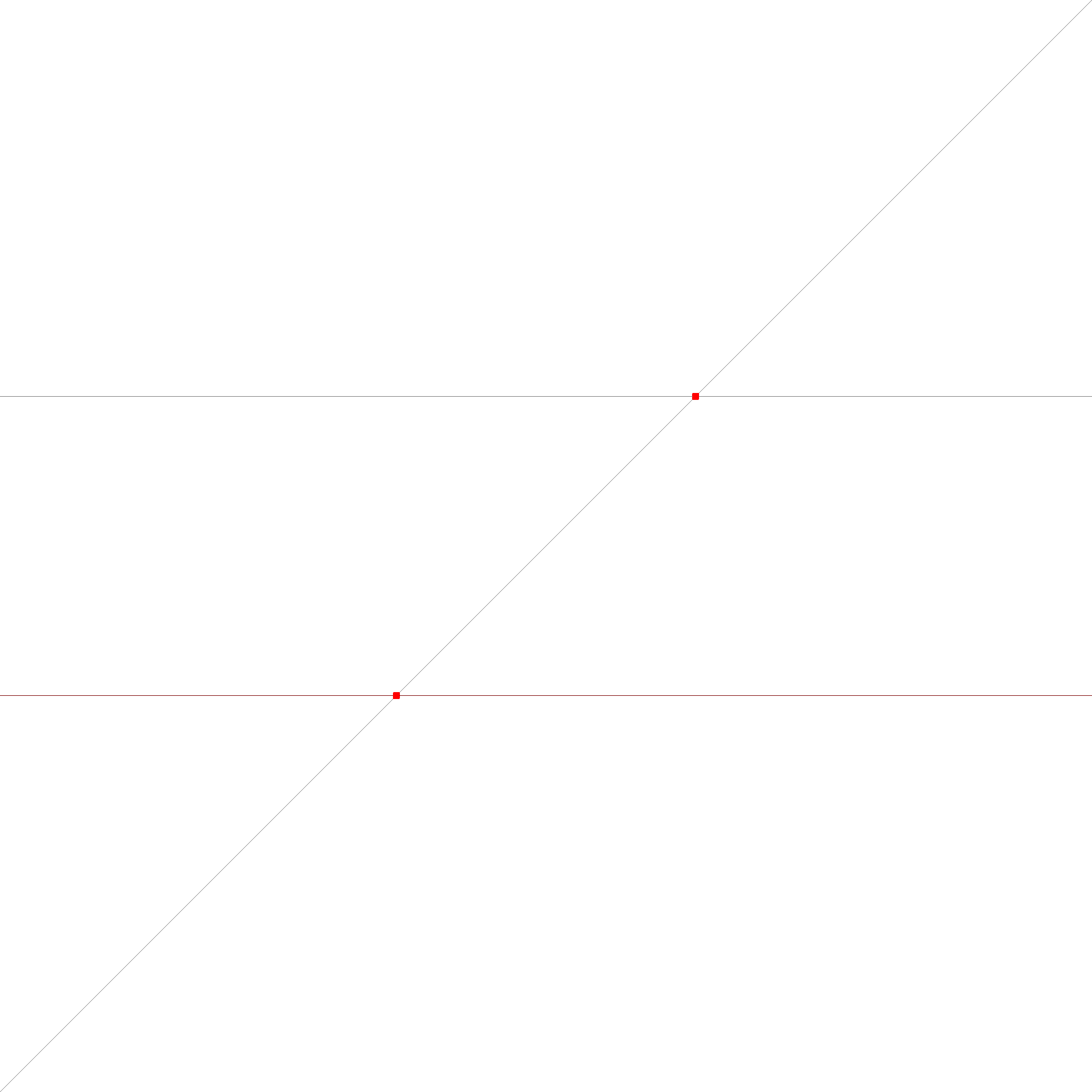
Here is an example of the intersection of multiple lines with each other. The intersections are red, the lines are black. Two black lines overlap each other and result in a red line. The other lines intersect only in the red points.

Line Intersections

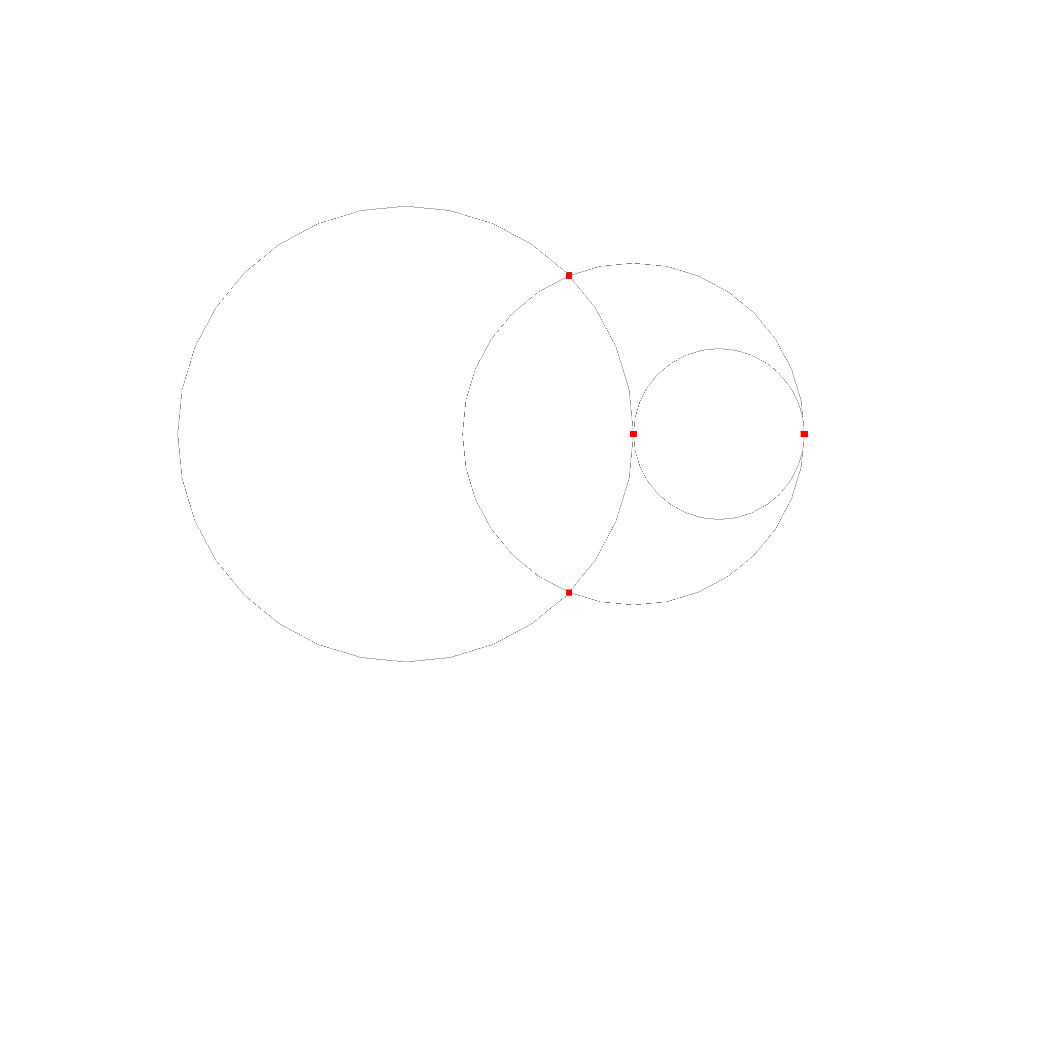
These are the intersection cases for circles. The circles are black, the intersections are red. Two circles overlap and result in a circle. Two other circles intersect in two points. The last case is where the circles just touch each other and intersect in one point.

Circle Intersections

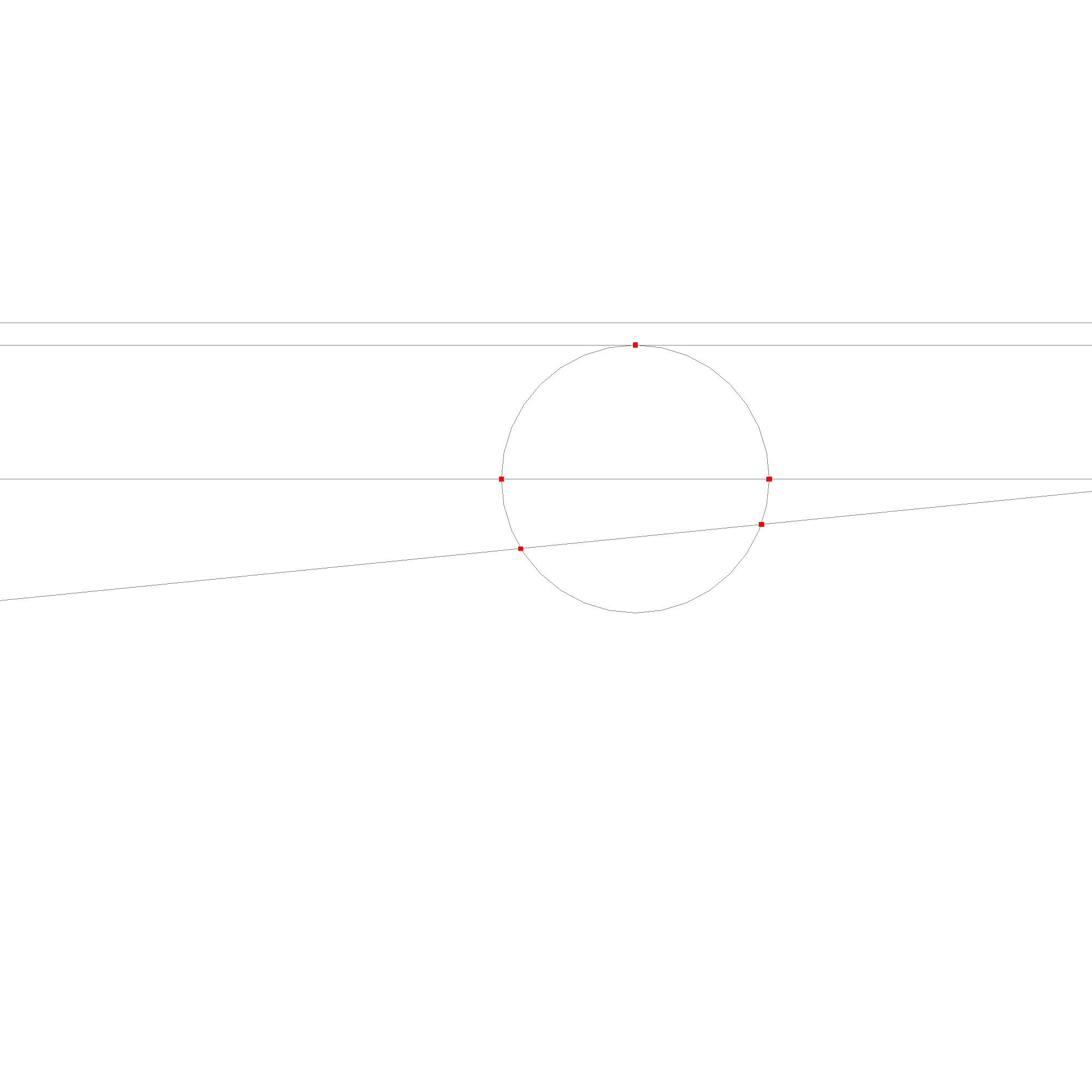
The last case is the intersection of a line and a circle.

Line Circle Intersections

For ellipses, we use a numerical method to find the intersections.

Ellipse Intersections

Note: Implementation detail. The individual cases are implemented as circle_circle_intersection, circle_line_intersection and line_line_intersection. They are not a part of class, since it would not be clear in which class they should reside. We list them in alphabetical order. Then there is the Curve enum and a curve_curve_intersection function, which can be used for the general case. The Curve enum is used to represent the different cases of the intersection.

Surfaces

In this chapter, we will discuss the representation of surfaces in the context of B-rep modeling. Surfaces include planes and spheres so far.

This is a plane, defined by a basis and 2 directions.

#![allow(unused)]
fn main() {
let plane = Plane::new(basis, u_slope, v_slope);
}

Plane

Next is a sphere, defined by a center and a radius, and if the normal is facing outwards.

#![allow(unused)]
fn main() {
let sphere = Sphere::new(basis, radius, true);
}

Sphere

There is also a cylinder, which is defined by a basis, an extent direction, and a radius. The cylinder is infinite in the extent direction.

#![allow(unused)]
fn main() {
let cylinder = Cylinder::new(basis, extent, radius);
}

Cylinder

Interacting with Surfaces

How do we interact with surfaces? We can do this by using the Surface trait. It implements the following methods:

#![allow(unused)]
fn main() {
// Transforms the surface by the given transform.
pub fn transform(&self, transform: Transform) -> Surface;

// Change normal direction of the surface.
pub fn neg(&self) -> Surface;

// Returns the normal of the surface at point p.
pub fn normal(&self, p: Point) -> Point;

// Checks if the point p is on the surface.
pub fn on_surface(&self, p: Point) -> bool;

// Returns the Riemannian metric between u and v
pub fn metric(&self, x: Point, u: TangentPoint, v: TangentPoint) -> f64;

// Returns the Riemannian distance between x and y.
pub fn distance(&self, x: Point, y: Point) -> f64;

// Exponential of u at base x. u_z is ignored.
pub fn exp(&self, x: Point, u: TangentPoint) -> Point;

// Log of y at base x. Z coordinate is set to 0.
pub fn log(&self, x: Point, y: Point) -> Option<TangentPoint>;

// Parallel transport of v from x to y.
pub fn parallel_transport(
    &self,
    v: Option<TangentPoint>,
    x: Point,
    y: Point,
) -> Option<TangentPoint>;

// Returns the geodesic between p and q.
pub fn geodesic(&self, x: Point, y: Point) -> Curve;

// Returns a point grid on the surface, which can be used for visualization.
pub fn point_grid(&self, density: f64) -> Vec<Point>;

// Finds the closest point on the surface to the given point.
pub fn project(&self, point: Point) -> Point;
}

Riemannian Manifolds

We model surfaces as Riemannian manifolds. A Riemannian manifold is a smooth manifold with a Riemannian metric. The Riemannian metric is a positive-definite symmetric bilinear form on the tangent space at each point that varies smoothly from point to point. The Riemannian metric allows us to measure distances and angles on the surface. If the inner product is 0, the vectors are orthogonal. If the inner product is positive, the vectors are aligned in the same direction. If the inner product is negative, the vectors are aligned in the opposite direction.

Dont be scared, there is a simple way to think about this. Riemannian manifolds allow us to convert 3d problems into 2d problems. Many algorithms like for example the ray check algorithm to check if a point is inside a face, or delauany triangulation, or the voronoi diagram, are much easier to implement in 2d. Using Riemannian manifolds, we can convert these problems into 2d problems, as long as we find a reference point where each point we are working with is "close enough" to.

Geodesics

One very important function we need are geodesics. They are the shortest path between two points on the surface. We can use them to find the distance between two points, or to find the closest point on the surface to a given point.

Geodesic

Do you see how the lines connect the points in the shortest way possible while also following the surface exactly? Thats what geodesics are. They are supported for all surface types, take a look at the cylinder geodesic for example:

Cylinder Geodesic

The geodesic of a cylinder is a helix.

Exponential and Logarithmic Maps

Another feature we use very often are the exponential and logarithmic maps. Very roughly, we can use them to flatten out points on a 3D surface to a 2D plane, and then later to map them back to the surface. This is very useful for example when we want to rasterize a surface, or when we want to find the closest point on the surface to a given point.

Exponential and Logarithmic Maps

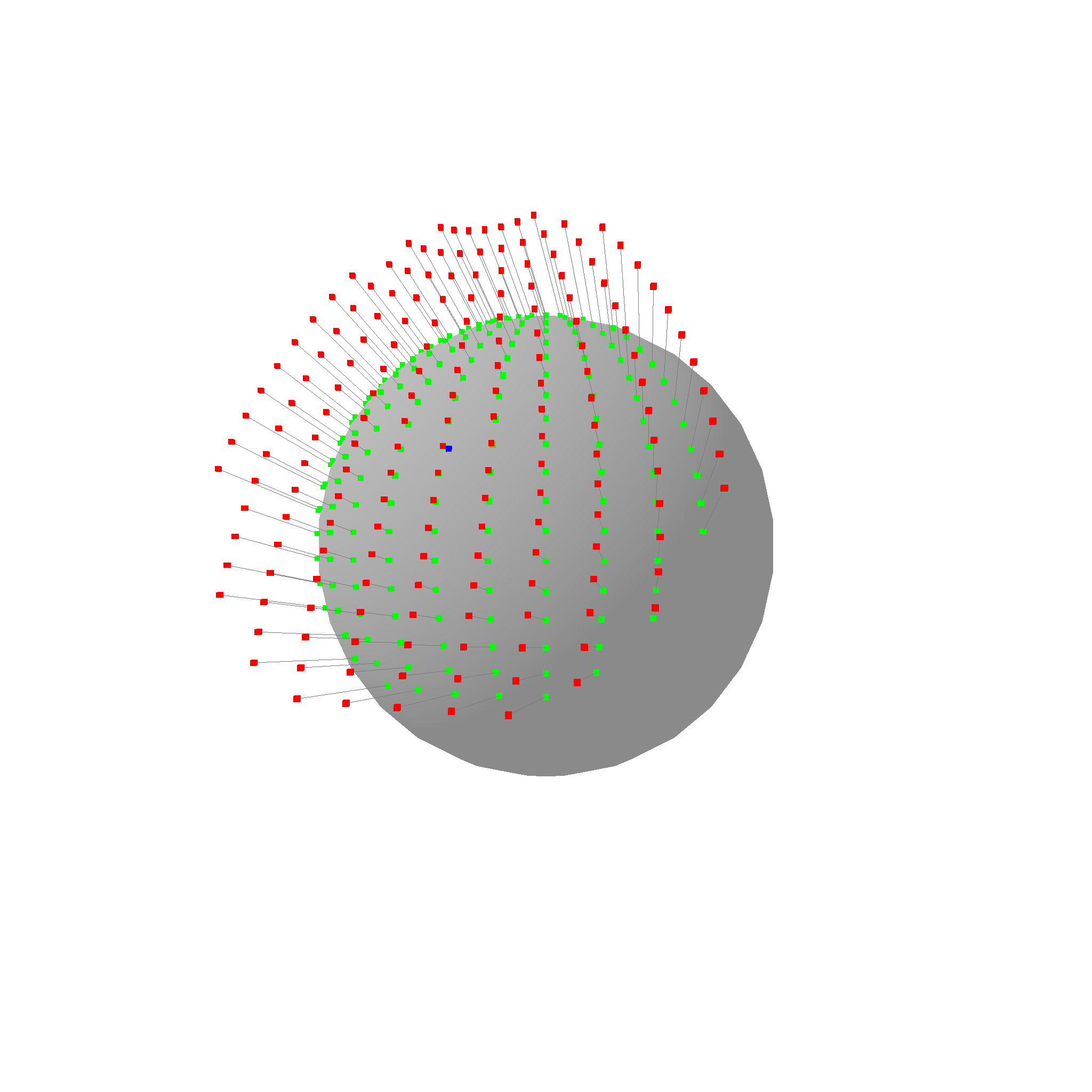
Note: For visualization purposes, the red points are shifted to the anchor point. In reality, the plane of the red points goes through the origin, not the anchor point.

Are you able to see how the green points on the sphere are mapped to the red points on a plane? The logarithmic map is the function that maps the red points back to the green points. The exponential map is the function that maps the green points to the red points. This is a very powerful tool to convert 3d problems into 2d problems.

The logarithmic map is not always defined. For example, the logarithmic map is not defined at the opposite pole of a sphere. In this case, the logarithmic map returns None. However, in close proximity to the anchor, the logarithmic map is well defined. Here is one more example of the logarithmic map:

Logarithmic Map

Intersections

We do support all sorts of intersections between curves and surfaces.

Curve-Curve Intersections

Curve Curve intersections result in one of three cases:

Intersection is a curve. This can only happen with two equal curves.
Intersection is a finite set of discrete points
Intersection is a infinite set of discrete points (this can happen between a helix and a line). This is just models as a PointArray, a set of equidistant points.
No intersection

#![allow(unused)]
fn main() {
pub enum CurveCurveIntersection {
    None,
    FinitePoints(Vec<Point>),
    InfiniteDiscretePoints(PointArray),
    Curve(Curve),
}
}

One very imporant thing to understand is that curve-curve intersections cannot result in something like a short edge and a point. The intersection is EITHER the same curve, OR a set of points. This follows from one of the fundamental properties of curves. The proof looks something along the lines of:

Let C1 and C2 be two curves.
Let P be an intersection point on C1 and C2.
Now do the taylor expansion of C1 and C2 around P.
Either the taylor expansions are equal, or they are not.
1. If they are equal, then C1 and C2 are the same curve.
2. If they are not equal, then there is an infinitly small neighborhood around P where C1 and C2 are not equal, hence P is a discrete intersection point.

Similar proofs can be made for surfaces etc. You can look it up under Bézout's theorem.

Curve-Surface Intersections

...

Chapter 3 Topology

Infinite lines and planes are great, but also fairly limiting. We want to manufacture more than infinite planes and lines. We want to manufacture parts with holes, fillets, and other features. We want to manufacture parts with bounded surfaces and volumes. This is where topology comes in.

This crate has everything to define even complex geometries. It includes vertices, edges, faces and volumes. It also includes containment checks.

This is the numpy of CAD. Numpy is a Python library that defines a datastructure to store and manipulate n-dimensional arrays. It is the foundation of many scientific libraries in Python that use these arrays as a common language. This crate is the foundation of the modern-brep-kernel. It is like a STEP file and can represent any geometry. It itself however is not very useful, but other crates provide functions to create and manipulate these structures.

This is why boolean operations and rasterization are in separate crates. You can also create your own extension crates that define new operations on these structures like fillets, or part libraries that define standard parts like screws or nuts.

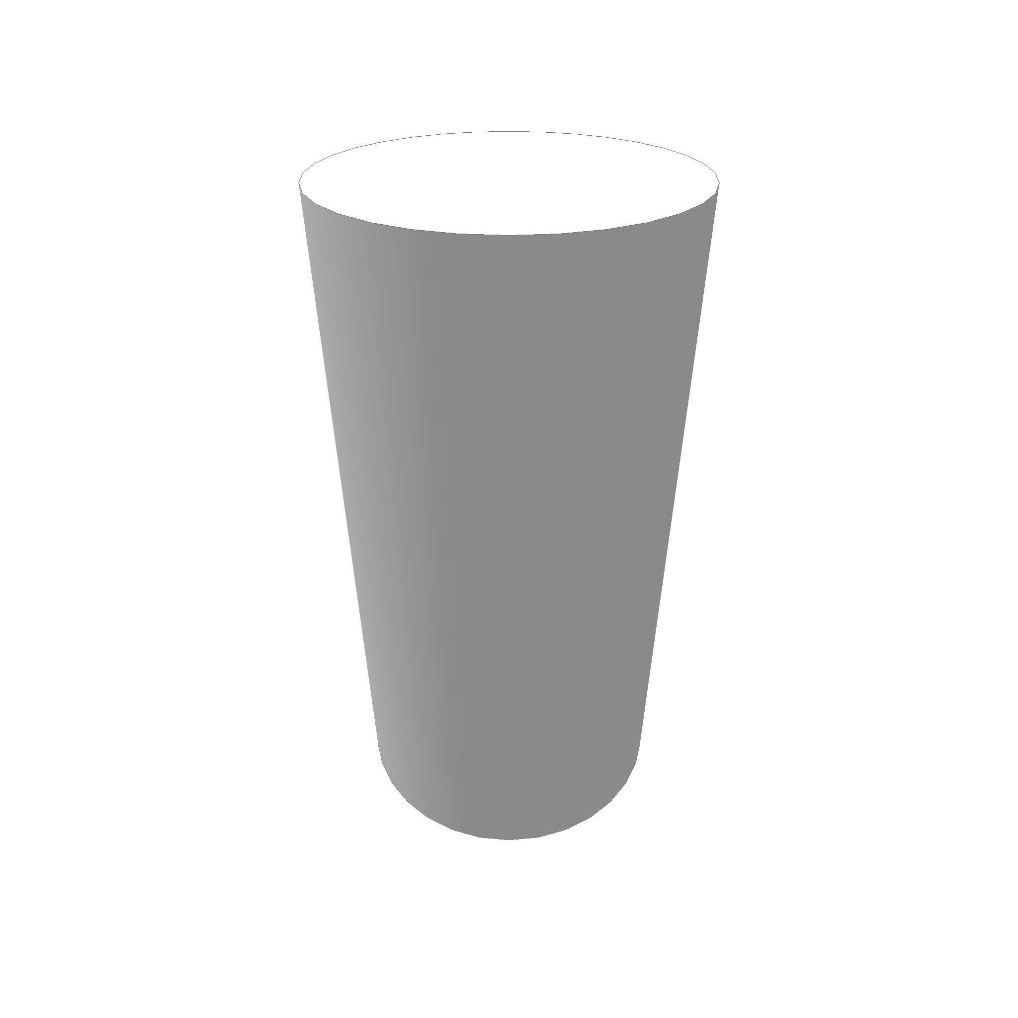
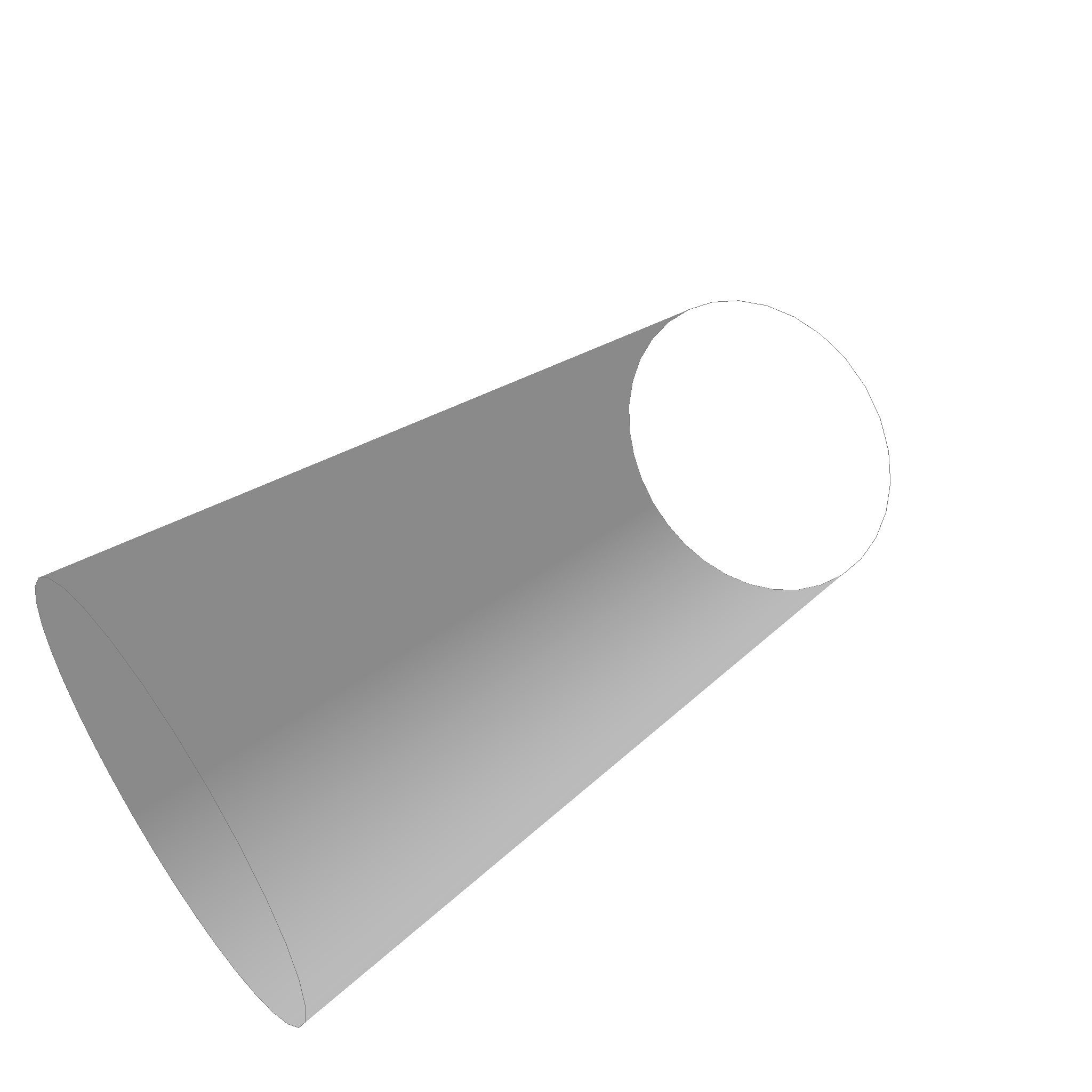
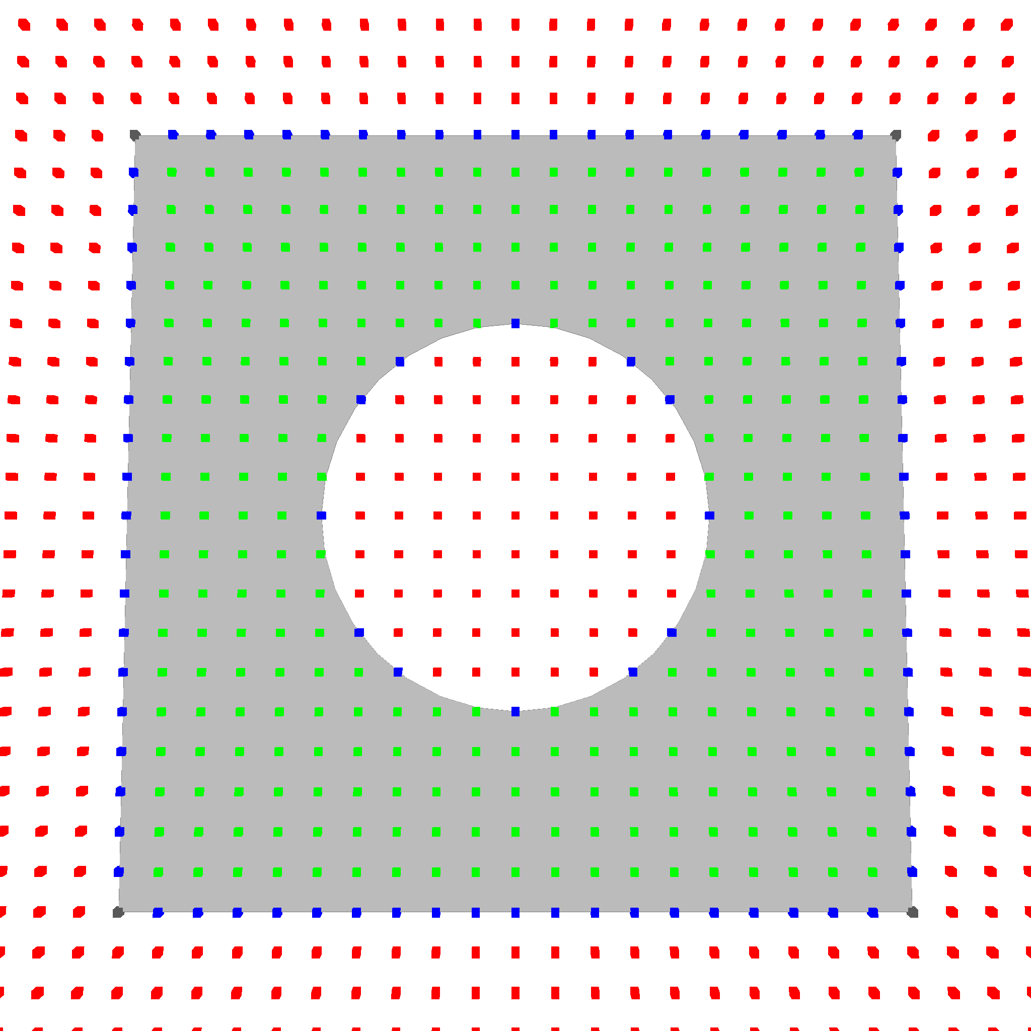
Edges

An Edge is defined by a base curve, and a possible start and end point.

#![allow(unused)]
fn main() {
pub struct Edge {
    pub start: Option<Point>,
    pub end: Option<Point>,
    pub curve: Curve,
}
}

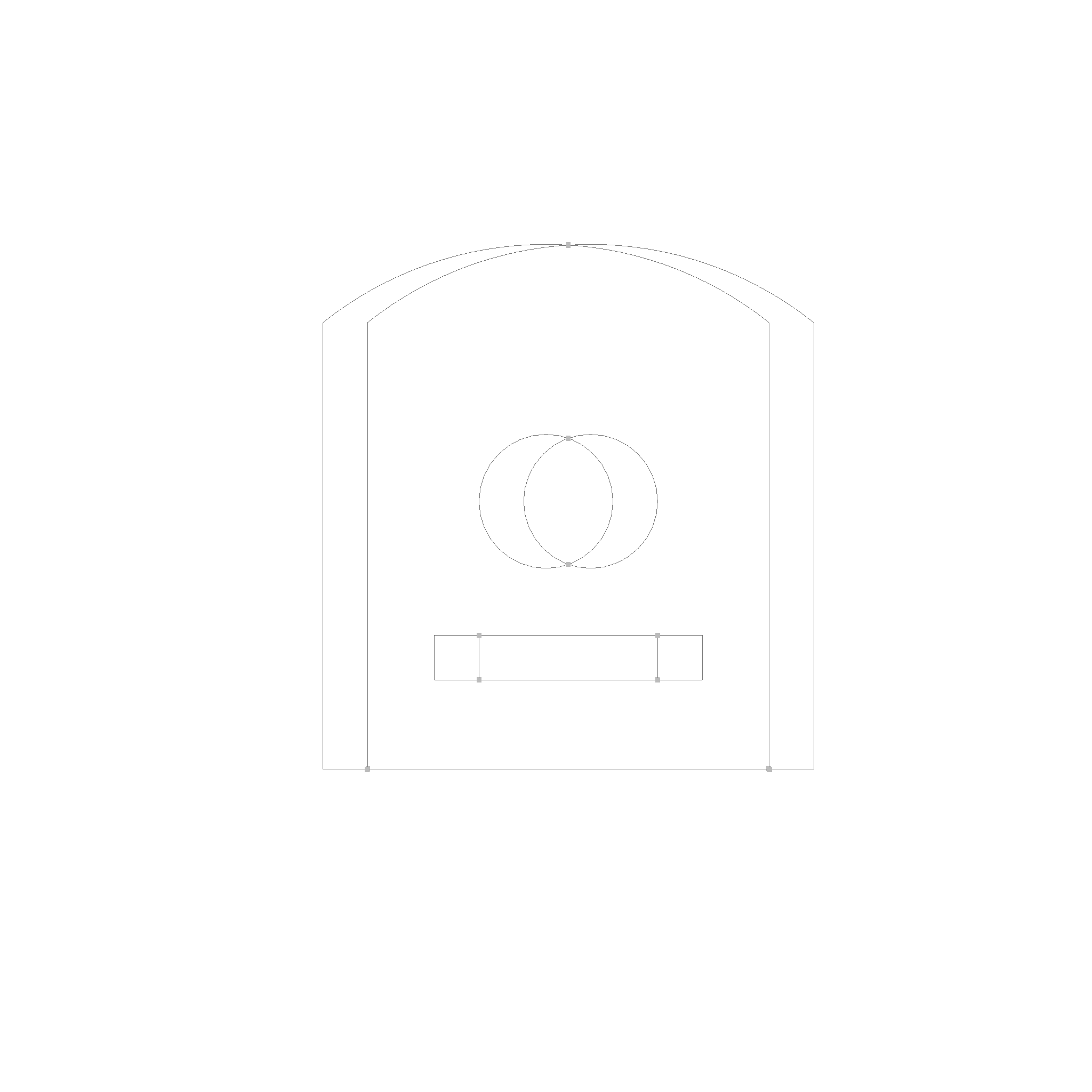
Here are some picture of various edges:

Edges

There is a line and a arc, which are bounded by start and end points. The circle is unbounded, so it has no start and end point.

Contours

A contour is a connected vector of edges. It is used to define the boundary of a face. A contour has to be closed, meaning that the first and last edge have to be the same.

#![allow(unused)]
fn main() {
pub struct Contour {
    pub edges: Vec<Edge>,
}
}

Contour

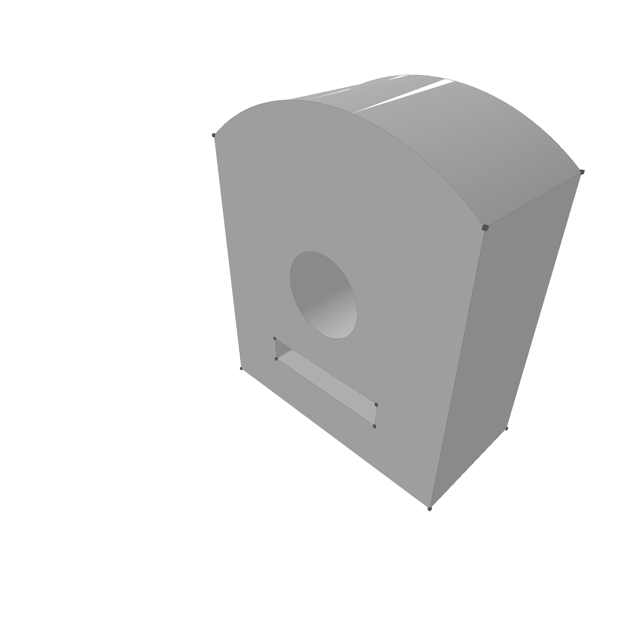
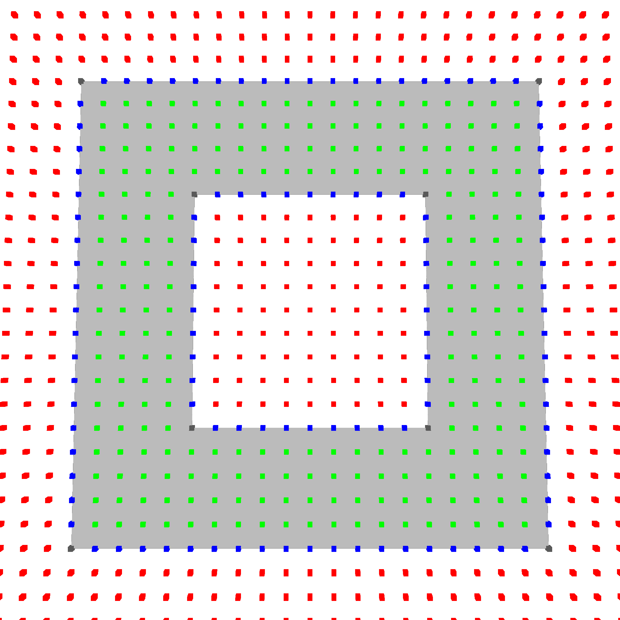
Faces

Faces are defined by a surface, and some contours for boundaries.

#![allow(unused)]
fn main() {
pub struct Face {
    pub boundaries: Vec<Contour>,
    pub surface: Rc<Surface>,
}
}

Wait a second... Shouldn't we have one outer boundary that is counter clockwise, and multiple holes that are clockwise. Yes, for simple shapes like planar cutouts this works, but it is in general not clear which ones of all the boundaries is the outer one. For example, if you have a cylinder, you can choose the top or the bottom as the outer boundary. This is why we have a list of boundaries, and the first one is the outer boundary. The only thing that is important is that the face is one continous patch of space, not multiple. This is assumed in the following algorithms.

A face can look something like this:

Face

In wireframe mode, you see how the face is triangulated for rendering

Face Wireframe

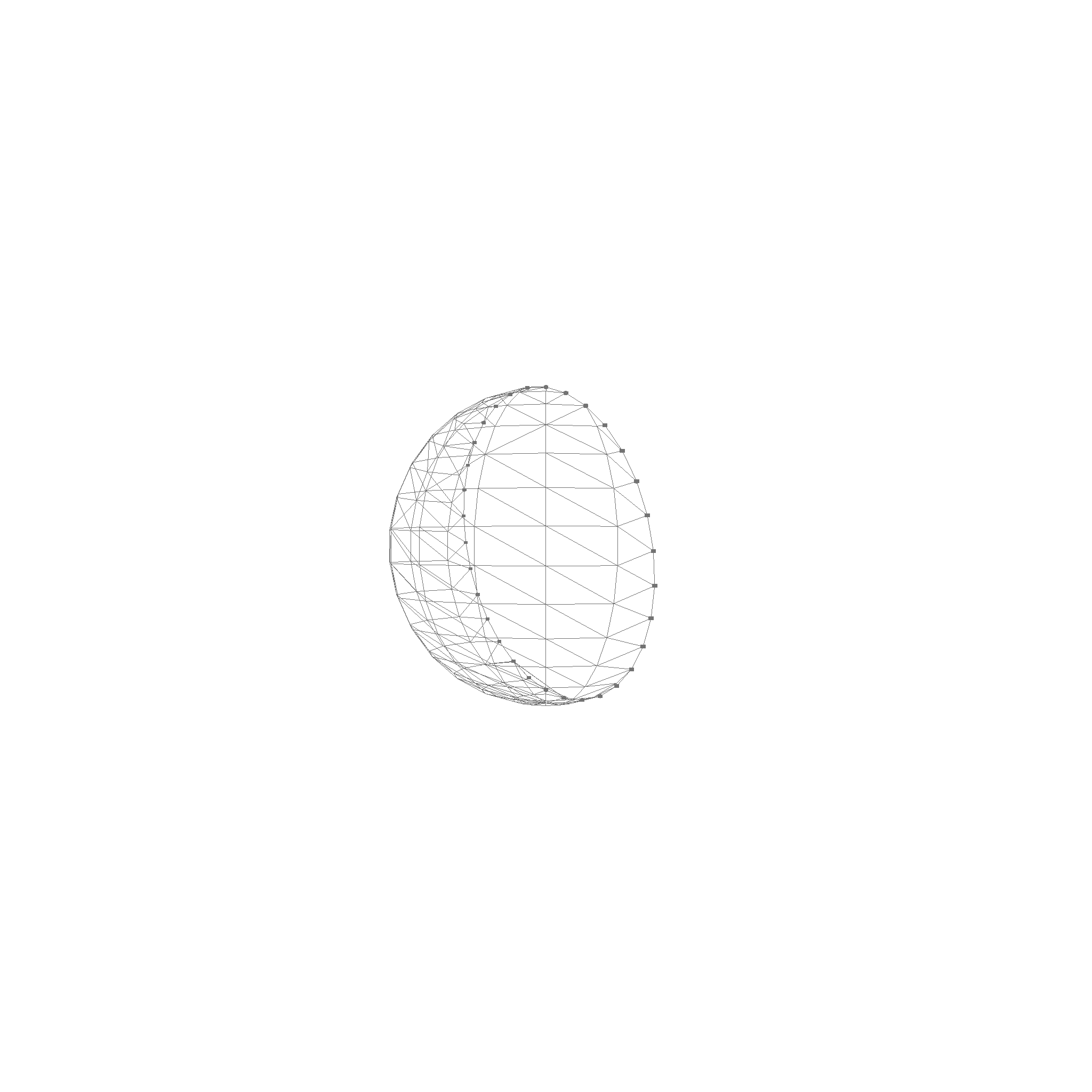
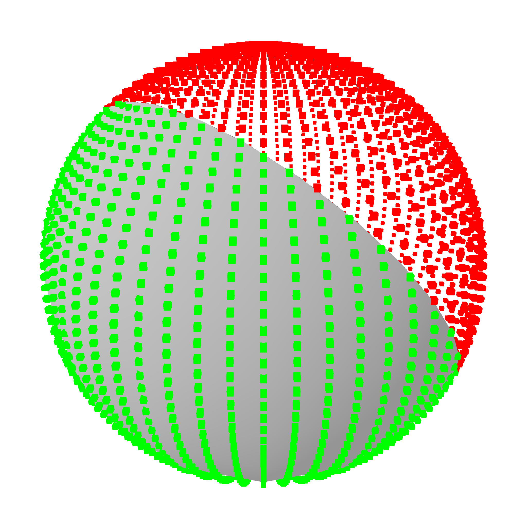
Faces can also be non-planar, like this half sphere:

Face Half Sphere

In wireframe mode, you see how the face is triangulated for rendering

Face Half Sphere Wireframe

Here are some cylinder faces. The cylinder is interesting, because it has a boundary and a hole, but we can choose which one is which. The top, or the bottom ring can be the boundary, with the other being the hole.

Face Examples

Face With Hole

Shells

Shells are a collection of faces that together form a closed space. They have to be watertight, meaning that there are no holes in the shell. This does not mean a shell cannot represent a drill hole, but that the inner side of the drill hole is also represented by a face.

#![allow(unused)]
fn main() {
pub struct Shell {
    pub faces: Vec<Face>,
}
}

Shell

Shell2

Volumes

A volume defined by a shell, which is the boundary of the volume. Additionally, it can have cavities, which are also defined by a shell.

#![allow(unused)]
fn main() {
pub struct Volume {
    pub boundary: Shell,   // Normal pointing outwards
    pub cavities: Vec<Shell>, // Normal pointing inwards
}
}

Caveties are only visible in cross-section view, which is not yet implemented.

Shell

Containment

The crate also allows for containment checks for every topological structure. They work by ray casting and checking the normal at the intersection with the boundary. This also works for edge cases when the casted ray hits a corner.

This works for various faces. Red means outside, green means inside, blue means on the edge, and gray means on the corner.

Containment

And also for various volumes.

TODO: Add images

Why cant we just count the intersections?

Imagine we are at a corner of a contour. We want to check if a point is inside or outside the contour. We can do this by drawing a line from the point to the corner (ray). If the line crosses the contour an odd number of times, the point is inside the contour. If the line crosses the contour an even number of times, the point is outside the contour.

However, this method is not perfect. If we pass through a corner, the method might miscount the number of intersections. So we have to make sure we do not pass through a corner.

Edge case

Alternatifly, we can also take a look at the direction of the closest intersection. If we normalize -ray, -tangent_1 and tangent_2, if -ray is on the top side of the green dashed line, we know it comes from inside. We can also create a coordinate system (red lines and normal) and check its handedness. It switches handed ness when -ray is crossing the contour. This is a more robust method, fully deterministic and deals with the edge case.

Inside or Outside

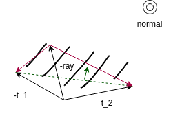
A common idea is also to check the normals. If the ray is $n \cdot d$ is positive for both normals $n$ and the direction of the ray $d$, we know we are inside the contour. This is true. But depending on if it is a concave or convex corner, it is sufficient that one of the dot products is positive (area 2 and 4), or both have to be positive (area 1).

Inside or Outside

Three dimensional case

Same idea. If the coordinate system changes handedness, we know we are inside the corner. Inside or Outside

Rasterization

Most stuff is pretty easy to rasterize. Just creating watertight faces is a bit thougher.

The first step is to rasterize the edges. This will ensure that all faces are bounded by the exact same edge vertices.

Then we generate a point grid on the surface and filter out all points that are not inside the face.

Then we use delauny triangulation.

Rasterization

Boolean Operations

Boolean operations are pretty complex. This crate implements 2d and 3d booleans based on the datastructure.

What makes this so tricky is that there are a lot of cases where lines are parallel or overlapping and so on. In most software they are edge cases and occur rarely, but for a CAD kernel they occur quite frequently. Take for example a face that is extruded until it reaches another face, and then you want to compute the union. This is a very common operation in CAD software. Treating this correctly is very important.

In general, they work by splitting the faces at the intersection points and then filtering out the parts that are inside or outside the other face. Then the parts are reassembled.

Boolean Face Operations

2D boolean operations are fully supported.

The first step is to find all split points. These are points where the boundaries intersect, or start to intersect, or end to intersect.

The next step is to split the curves at these points into segments, which are then categorized into 8 categories. Based on these categories, the segments are then filtered out. Take for example the filter for the intersection function.

#![allow(unused)]
fn main() {
FaceSplit::AinB(_) => true,
FaceSplit::AonBSameSide(_) => true,
FaceSplit::AonBOpSide(_) => false,
FaceSplit::AoutB(_) => false,
FaceSplit::BinA(_) => true,
FaceSplit::BonASameSide(_) => false,
FaceSplit::BonAOpSide(_) => false,
FaceSplit::BoutA(_) => false,
}

By checking if the midpoint of each edge is inside, outside, or on the boundary of the other face, we can determine which edges have to stay for the intersection operation. The following picture shows each category in a different color in an exploded view.

Then the segments are reassembled into new contours. The contours are then sorted into a hierarchy and the faces are reassembled.

This is the result of the intersection operation.

This is the result of the union operation.

This is the result of the difference operation.

Boolean Solid Operations

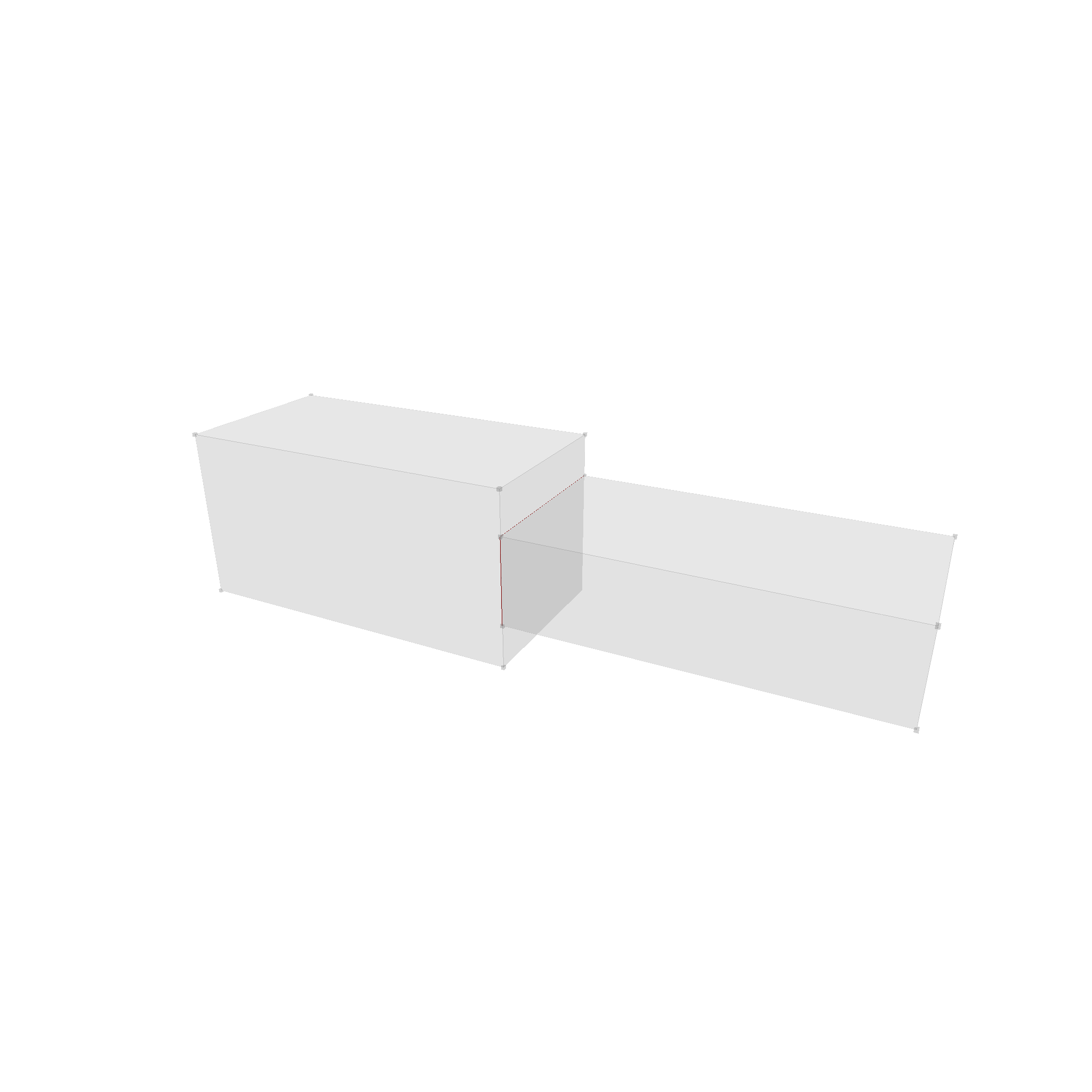
3D booleans work in a similar way to 2D booleans. The first step is to find all split edges. To find these, we compare each pair of Faces and find the intersection. If the intersection is a point, we ignore it. If the intersection is a line, we add it to the list of split edges. If the intersection is a face, all boundary edges are also added to the list of split edges.

In red, you can see the split edges. Due to clipping, only 2 of the 4 split edges are visible.

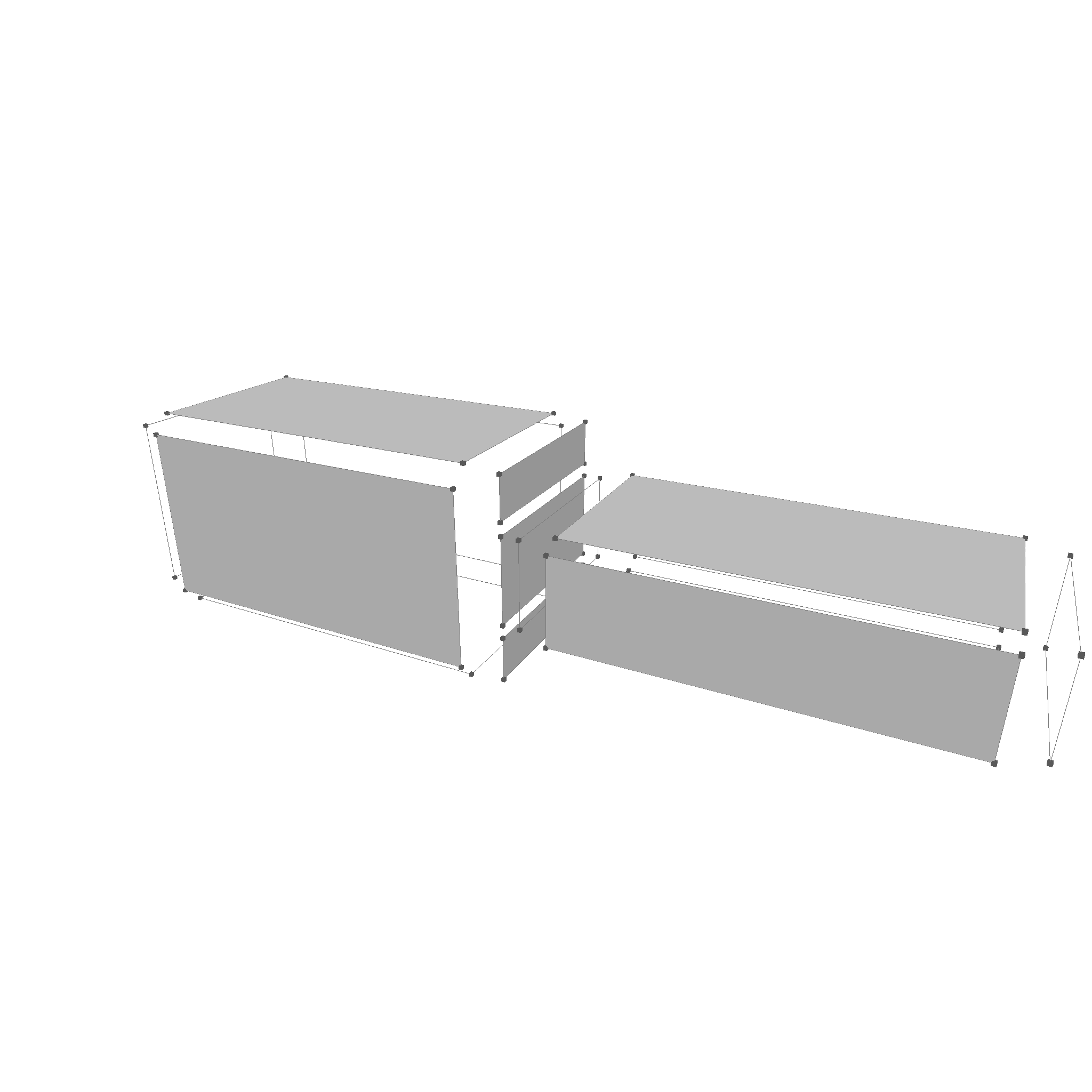
The next step is to split each face along all possible split edges. To do this, we iterate over all faces and edges, and split the face by the edge if necessary. This is the most complex part of the boolean operation. Some edge cases that have to be considered are:

In general, we have to split the face boundaries at the start and end of the edge.
Now the behavior depends on of the start and end of the edge actually lie on the face boundary.
- If none lies on the boundary, a new hole is created.
- If only one lies on the boundary, the boundary is extended with a new path back and forth.
- If both lie on the boundary, it depends.
  - If its the same boundary, split it into two faces.
  - If its different boundaries, connect them back and forth, and make them one boundary.

This leads to the following result

The next step is to use an inner point on the surface to determine if a face is inside, outside, equal with normals facing in the same direction, or equal with normals facing in the opposite direction. Determining if an point is inside, outside or on the face of a volume is a simple test which can be made using a ray casting algorithm.

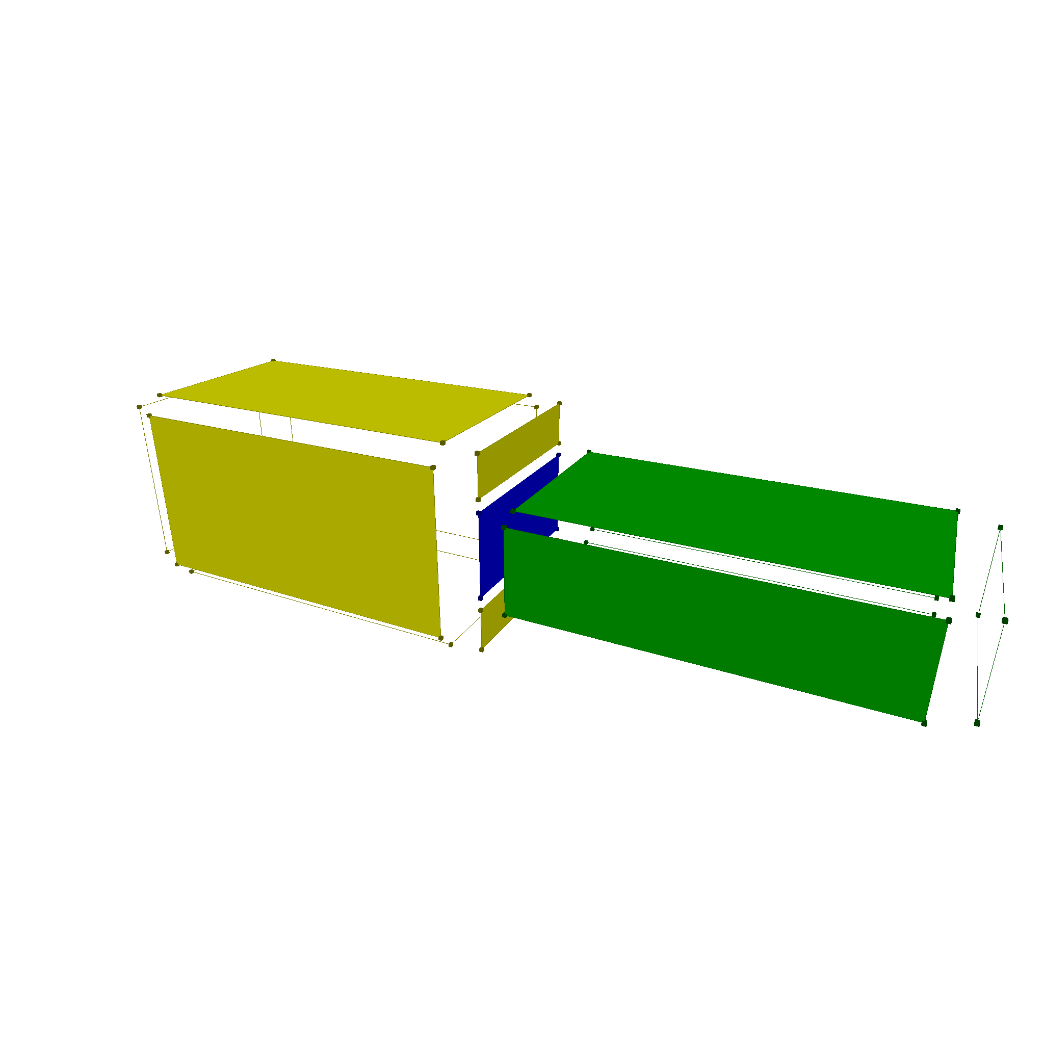
Now, depending on which class the faces fall into, we can determine the final result of the boolean operation. For example, for a union operation, we can use the following rules:

#![allow(unused)]
fn main() {
    VolumeSplit::AinB(_) => false,
    VolumeSplit::AonBSameSide(_) => true,
    VolumeSplit::AonBOpSide(_) => false,
    VolumeSplit::AoutB(_) => true,
    VolumeSplit::BinA(_) => false,
    VolumeSplit::BonASameSide(_) => false,
    VolumeSplit::BonAOpSide(_) => false,
    VolumeSplit::BoutA(_) => true,
}

This results in

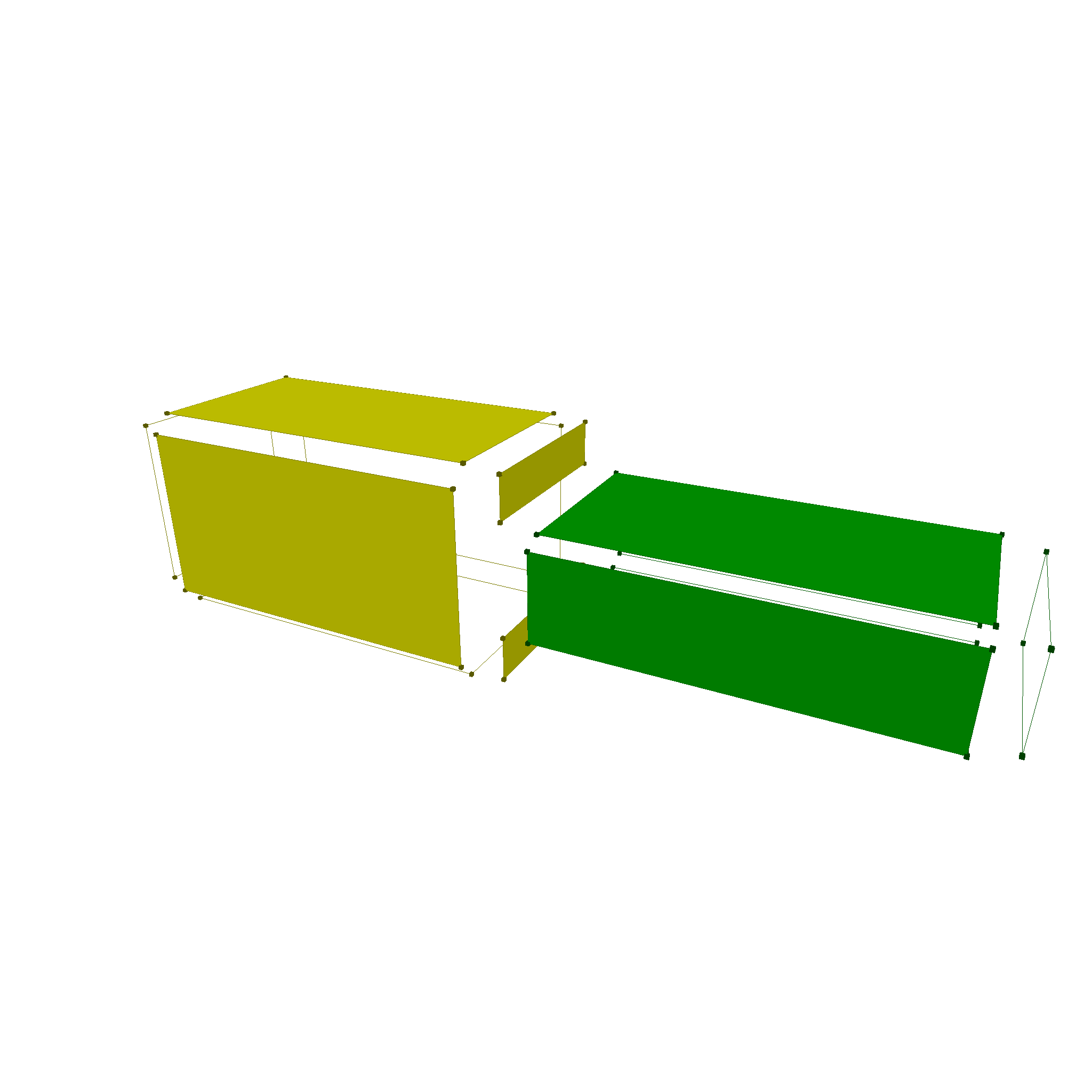
Now, the last step is to stich the faces back together to form shells, and then connect them back to a volume.

FAQ

Why not expose the parameter space of curves and surfaces?

Usually, the nasty details of the exact representation of a curve or surface should remain in geop-geometry. The other crates only interface to it via methods, where instead of a parameter, a 3d point is used.

E.g. for a curve, the function signature is not tangent(f64) -> Vec3, but tangent(Vec3) -> Vec3.

This may have performance implications for functions, where projection is expensive. In the future, we might use the plane, cylinder and sphere as prototypical parameter spaces. So far, however, those functions are only called in places where a projection would be necessary anyway, so there is no performance loss yet. And for simple cases, like a sphere, the normal(Vec3) -> Vec3 function is even faster than normal(f64, f64) -> Vec3.

Why not use the half-edge data structure?

So far, this datastructure has not been necessary. It also contradicts the "single source of truth" principle.

The problem is, that each operation now has to make sure that the next edge, the previous edge is pointing to, points back to the current edge. If just one operation in all of geop-geometry forgets to update this, the whole system breaks down.

Instead, edges are bound by points, which are checked every time an edge is created. For face boundaries, it is also checked that the edges are connected in the right order.

If you have an algorithm that is much faster with the half-edge data structure, it would be possible to implement it in a separate crate, and treat it as a "cache" layer for the actual data. This is similar for example to how the internet works. The actual data is stored in a database, and a cache layer is used to speed up access.

Why are faces constrained by 3d edges, not by 2d edges in parameter space?

Two touching faces have to be bound by the same edge in 3d space. This is useful for watertight meshes. Geop generates watertight meshes, because first the edges are rasterized, then the inner parts of the faces, and then the gap is bridged.

It becomes more interesting in cases, where the face boundaries can only be approximated. Doing this in parameter space might seem easier at first glance, but there will still be a point in time where the 3d edge has to be created, and projected back to the parameter space of the second face. So there is not really a performance gain.

For surfaces like a sphere, the 3d edge is always well defined. It can be easily bound by circles for example. A 2d boundary in the spheres parameter space however degenerates at the poles, which would make intersection algorithms hard to implement.

Is the border of a face still part of the face?

Good question. In general, no. Even though this might be subject to change.

So for example, the intersection of two touching faces is empty.

The intersection of a line touching a face (from outside) is 2 lines, which end and start at the touching point. This is useful for the boolean operations, as it creates a split point.

However, when checking if a point is inside a face or an edge, the function will tell you if it is actually inside, on the boundary, or outside.

\( B_{i,j}(x) \)	Expression
\( B_{0,0}(x) \)	\( 1.00 \cdot x^0 \)
\( B_{0,1}(x) \)	\( -1.00 \cdot x^1 + 1.00 \cdot x^0 \)
\( B_{1,1}(x) \)	\( 1.00 \cdot x^1 \)
\( B_{0,2}(x) \)	\( 1.00 \cdot x^2 - 2.00 \cdot x^1 + 1.00 \cdot x^0 \)
\( B_{1,2}(x) \)	\( -2.00 \cdot x^2 + 2.00 \cdot x^1 \)
\( B_{2,2}(x) \)	\( 1.00 \cdot x^2 \)
\( B_{0,3}(x) \)	\( -1.00 \cdot x^3 + 3.00 \cdot x^2 - 3.00 \cdot x^1 + 1.00 \cdot x^0 \)
\( B_{1,3}(x) \)	\( 3.00 \cdot x^3 - 6.00 \cdot x^2 + 3.00 \cdot x^1 \)
\( B_{2,3}(x) \)	\( -3.00 \cdot x^3 + 3.00 \cdot x^2 \)
\( B_{3,3}(x) \)	\( 1.00 \cdot x^3 \)
\( B_{0,4}(x) \)	\( 1.00 \cdot x^4 - 4.00 \cdot x^3 + 6.00 \cdot x^2 - 4.00 \cdot x^1 + 1.00 \cdot x^0 \)
\( B_{1,4}(x) \)	\( -4.00 \cdot x^4 + 12.00 \cdot x^3 - 12.00 \cdot x^2 + 4.00 \cdot x^1 \)
\( B_{2,4}(x) \)	\( 6.00 \cdot x^4 - 12.00 \cdot x^3 + 6.00 \cdot x^2 \)
\( B_{3,4}(x) \)	\( -4.00 \cdot x^4 + 4.00 \cdot x^3 \)
\( B_{4,4}(x) \)	\( 1.00 \cdot x^4 \)
...	...

Curve 1	Curve 2	Roots to find
Implicit \(u_1, u_2\)	Implicit \(v_1, v_2\)	\(u_1(x, y, z) = 0, u_2(x, y, z) = 0, v_1(x, y, z) = 0, v_2(x, y, z) = 0\)
Implicit \(u_1, u_2\)	Explicit \(p(t_2)\)	\(u_1(p(t_2)) = 0, u_2(p(t_2)) = 0\)
Explicit \(p(t_1)\)	Explicit \(p(t_2)\)	\(p(t_1) - p(t_2) = 0\)

Curve 1	Surface 2	Roots to find
Implicit \(u_1, u_2\)	Implicit \(v_1\)	\(u_1(x, y, z) = 0, u_2(x, y, z) = 0, v_1(x, y, z) = 0\)
Implicit \(u_1, u_2\)	Explicit \(p(t_2, t_3)\)	\(u_1(p(t_3, t_4)) = 0, u_2(p(t_3, t_4)) = 0\)
Explicit \(p(t_1)\)	Implicit \(v_1\)	\(v_1(p(t_1)) = 0\)
Explicit \(p(t_1)\)	Explicit \(p(t_2, t_3)\)	\(p(t_1) - p(t_2, t_3) = 0\)

Surface 1	Surface 2	Roots to find
Implicit \(u_1\)	Implicit \(v_1\)	\(u_1(x, y, z) = 0, v_1(x, y, z) = 0\)
Implicit \(u_1\)	Explicit \(p(t_3, t_4)\)	\(u_1(p(t_3, t_4)) = 0\)
Explicit \(p(t_1, t_2)\)	Explicit \(p(t_3, t_4)\)	\(p(t_1, t_2) - p(t_3, t_4) = 0\)

Modern BRep Kernels and CAD